for文を無くして高速化したいがfor文の方が速い
こちらのPythonのコードのデモデータ生成部分をR言語で再現したい。
https://github.com/tkEzaki/data_visualization/blob/main/8%E7%AB%A0/8_1_4_legend_examples.py
import pandas as pd  # データフレーム操作のためのPandas
import numpy as np  # 数値計算のためのNumPy

np.random.seed(0)  # 乱数のシードを固定

# 月曜日から日曜日までの7日間
days_of_week = ['月', '火', '水', '木', '金', '土', '日']

# 各時刻
hours_of_day = [10, 11, 12, 13, 14, 15, 16, 17, 18, 19, 20]

# データフレームを作成
df_visitor_count = pd.DataFrame(index=days_of_week, columns=hours_of_day)

# パターンに基づいて来客数を生成する関数(水曜日の特別処理を含む)
def generate_visitor_count_with_wednesday(day):
    visitor_count = []
    for hour in hours_of_day:
        if day == '水':
            # 水曜日は12時と17時以外の時間に、普段の平日より1.5倍の来客
            if hour == 12 or hour == 17:
                visitor_count.append(np.random.randint(50, 80))
            else:
                visitor_count.append(int(np.random.randint(20, 50) * 1.4))
        elif day in ['土', '日']:
            # 休日は11:00 - 17:00 までまんべんなく多い
            if 11 <= hour <= 17:
                visitor_count.append(np.random.randint(70, 100))
            else:
                visitor_count.append(np.random.randint(30, 60))
        else:
            # 平日は12時と17時が多い
            if hour == 12 or hour == 17:
                visitor_count.append(np.random.randint(50, 80))
            else:
                visitor_count.append(np.random.randint(20, 50))
    return visitor_count


# 各日、各時刻の来客数をパターンに基づいて生成
for day in days_of_week:
    df_visitor_count.loc[day] = generate_visitor_count_with_wednesday(day)
これをR言語にChatGPT君が直訳したものがこちら。
後でベンチマークをとる関係で全体を関数化しています。
fun_for <- function() {
  # 乱数のシードを固定
  set.seed(0)

  # 月曜日から日曜日までの7日間
  days_of_week <- c('月', '火', '水', '木', '金', '土', '日')

  # 各時刻
  hours_of_day <- c(10, 11, 12, 13, 14, 15, 16, 17, 18, 19, 20)

  # データフレームを作成
  df_visitor_count <- data.frame(matrix(ncol = length(hours_of_day), nrow = length(days_of_week)))
  colnames(df_visitor_count) <- hours_of_day
  rownames(df_visitor_count) <- days_of_week

  # パターンに基づいて来客数を生成する関数(水曜日の特別処理を含む)
  generate_visitor_count_with_wednesday <- function(day) {
    visitor_count <- c()
    for (hour in hours_of_day) {
      if (day == '水') {
        # 水曜日は12時と17時以外の時間に、普段の平日より1.5倍の来客
        if (hour == 12 || hour == 17) {
          visitor_count <- c(visitor_count, sample(50:80, 1))
        } else {
          visitor_count <- c(visitor_count, as.integer(sample(20:50, 1) * 1.4))
        }
      } else if (day %in% c('土', '日')) {
        # 休日は11:00 - 17:00 までまんべんなく多い
        if (11 <= hour && hour <= 17) {
          visitor_count <- c(visitor_count, sample(70:100, 1))
        } else {
          visitor_count <- c(visitor_count, sample(30:60, 1))
        }
      } else {
        # 平日は12時と17時が多い
        if (hour == 12 || hour == 17) {
          visitor_count <- c(visitor_count, sample(50:80, 1))
        } else {
          visitor_count <- c(visitor_count, sample(20:50, 1))
        }
      }
    }
    return(visitor_count)
  }

  # 各日、各時刻の来客数をパターンに基づいて生成
  for (day in days_of_week) {
    df_visitor_count[day, ] <- generate_visitor_count_with_wednesday(day)
  }
  # データフレームを準備
  df_plot <- data.frame(Hour = rep(hours_of_day, times = length(days_of_week)),
                        Day = rep(days_of_week, each = length(hours_of_day)),
                        Visitors = as.vector(t(df_visitor_count)))
しかし、for文を使うのはRらしくないし、sample関数で1個ずつ生成するのは如何にも効率が悪い。
そこでこんな風に書き直してみました。
sample関数は全期間分を一気に生成し、そこから条件に合ったものを取り出す形です。sample関数を何回も繰り返さない分高速化するでしょ! と思ってました。
fun_my <- function() {
  df_base <- expand_grid(
    days_of_week = c("月", "火", "水", "木", "金", "土", "日"),
    hours_of_day = 10:20
  )

  n <- nrow(df_base)

  set.seed(0)

  df_visitor_count <- df_base |>
    mutate(
      A = sample(50:80, n, replace = TRUE),       #水曜日のボーナスタイム(12時、17時)以外
      B = sample(20:50, n, replace = TRUE) * 1.5, #水曜日のボーナスタイム(12時、17時)
      C = sample(70:100, n, replace = TRUE),      # 土日の11:00-17:00
      D = sample(30:60, n, replace = TRUE),       # 土日の他の時間
      E = sample(50:80, n, replace = TRUE),       # そのほかの曜日のボーナスタイム(12時、17時)
      F = sample(20:50, n, replace = TRUE),       # そのほかの曜日のそのほかの時間
      visitor_count = case_when(
        days_of_week == "水" & !(hours_of_day %in% c(12, 17)) ~ A,
        days_of_week == "水" & hours_of_day %in% c(12, 17) ~ B,
        days_of_week %in% c("土", "日") & hours_of_day %in% 11:17 ~ C,
        days_of_week %in% c("土", "日") & !(hours_of_day %in% 11:17) ~ D,
        !(days_of_week %in% c("水", "土", "日")) & hours_of_day %in% c(12, 17) ~ E,
        !(days_of_week %in% c("水", "土", "日")) & !(hours_of_day %in% c(12, 17)) ~ F
      ),
      hours_of_day = hours_of_day,
      days_of_week = factor(days_of_week, levels = c("月", "火", "水", "木", "金", "土", "日"))
    ) |>
    dplyr::select(days_of_week, hours_of_day, visitor_count)
}
この二つの方法の実行速度をmicrobenchmarkで確認したのがこちら。
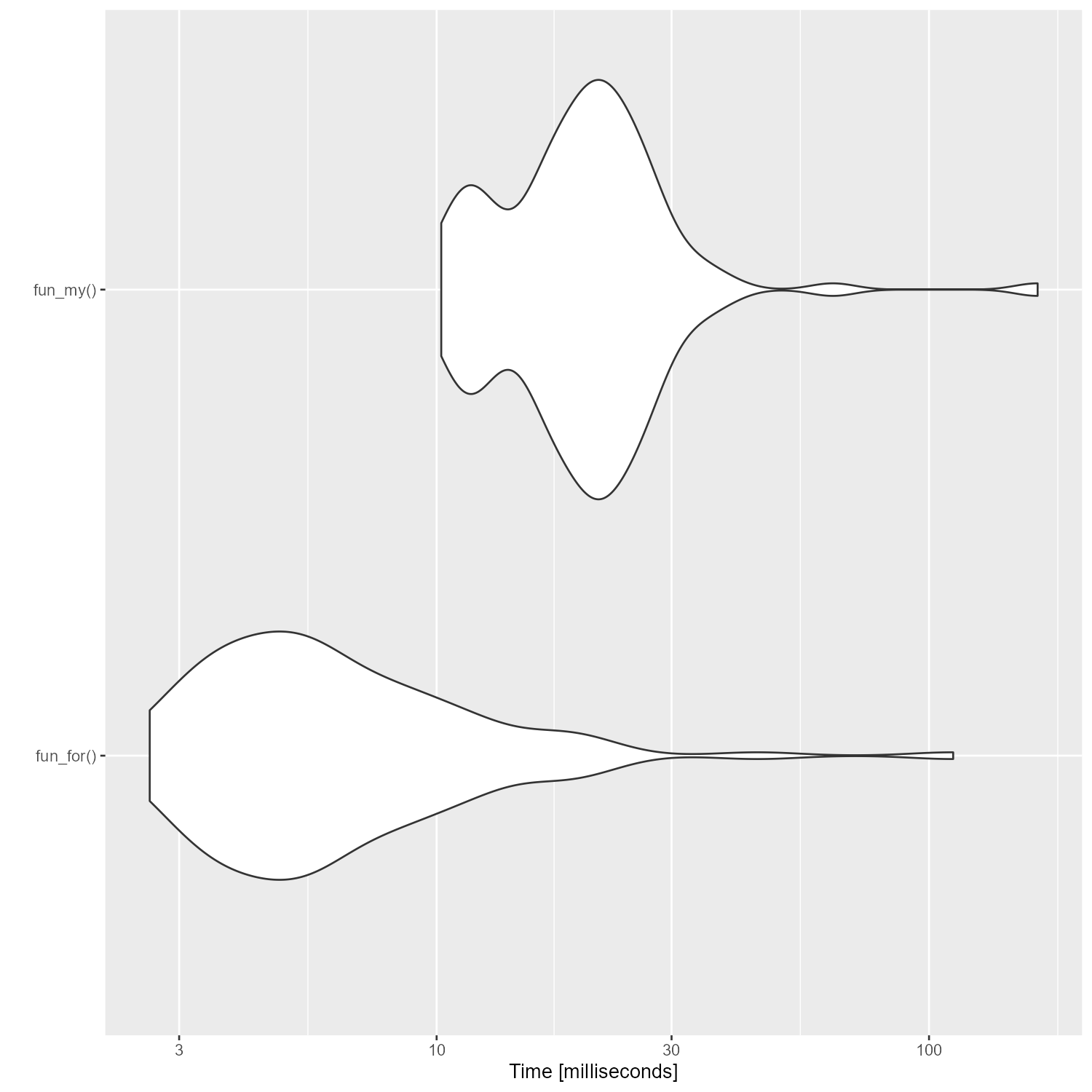
ぐぬぬ、直訳のfor文の方が速いじゃないか……
それでもfor文は使いたくないので試行錯誤した結果がこちら。
mutate()を無くしてtibble()でまとめる形にして、case_when()の中でsample()を使う形にしました。
fun_my3 <- function() {
  df_base <- expand_grid(
    days_of_week = c("月", "火", "水", "木", "金", "土", "日"),
    hours_of_day = 10:20
  )

  n <- nrow(df_base)

  set.seed(0)
  df_visitor_count <- tibble(
    days_of_week = factor(df_base$days_of_week, levels = c("月", "火", "水", "木", "金", "土", "日")),
    hours_of_day = df_base$hours_of_day,
    visitor_count = case_when(
      days_of_week == "水" & !(hours_of_day %in% c(12, 17)) ~ sample(50:80, 1),
      days_of_week == "水" & hours_of_day %in% c(12, 17) ~ sample(20:50, 1) * 1.5,
      days_of_week %in% c("土", "日") & hours_of_day %in% 11:17 ~ sample(70:100, 1),
      days_of_week %in% c("土", "日") & !(hours_of_day %in% 11:17) ~ sample(30:60, 1),
      !(days_of_week %in% c("水", "土", "日")) & hours_of_day %in% c(12, 17) ~ sample(50:80, 1),
      !(days_of_week %in% c("水", "土", "日")) & !(hours_of_day %in% c(12, 17)) ~ sample(20:50, 1)
    )
  )
}
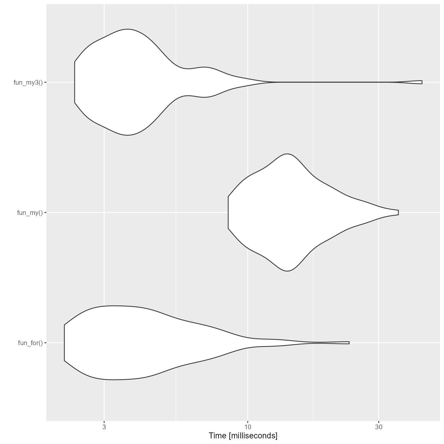
ベンチマークを取ると、なんとかfor文と同等の速さにはなった。
しかし、これは納得いかない。
どうすればfor文よりも高速化できるだろうか?
ネットワーク分析におけるコミュニティ抽出
この記事はR言語 Advent Calendar 2023 シリーズ2の18日目の記事です。
ネットワーク分析にコミュニティ抽出という手法があります。まあ、クラスター分析ですね。
Rのigraphパッケージには以下のコミュニティ抽出の方法が実装されています。
- ラベル伝播法 cluster_label_prop()
- ウォークトラップ cluster_walktrap()
- 辺媒介法 cluster_edge_betweenness()
- 貪欲アルゴリズム cluster_fast_greedy()
- スペクトラル最適化法 cluster_leading_eigen()
- 焼きなまし法 cluster_spinglass()
- インフォマップ法 cluster_infomap()
- ルーバン法 cluster_louvain()
- ライデン法 cluster_leiden()
どんなふうにコミュニティ抽出されるか試してみましょう。
ライブラリー呼び出し。
library(conflicted)
library(tidyverse)
library(igraph)
library(igraphdata)
有名な空手クラブのデータで試します。
data(karate)
karate |>
  plot()

コミュニティ抽出
cl_lp <- karate |> cluster_label_prop()# ラベル伝播法
cl_wt <- karate |> cluster_walktrap() # ウォークトラップ法
cl_eb <- karate |> cluster_edge_betweenness() # 辺媒介法
cl_fg <- karate |> cluster_fast_greedy() #貪欲アルゴリズム
cl_sp <- karate |> cluster_leading_eigen() #スペクトラル最適化法
cl_sg <- karate |> cluster_spinglass() |> with_seed(1234, code=_) # 焼きなまし法
cl_im <- karate |> cluster_infomap() |> with_seed(1234, code=_) # インフォマップ法
cl_lo <- karate |> cluster_louvain() |> with_seed(1234, code=_) # ルーバン法
cl_le <- karate |> cluster_leiden() |> with_seed(1234, code=_) #ライデン法
結果を描画
plot(cl_lp, karate, main = "ラベル伝播法", layout = layout_with_kk)
plot(cl_wt, karate, main = "ウォークトラップ法", layout = layout_with_kk)
plot(cl_eb, karate, main = "辺媒介法", layout = layout_with_kk)
plot(cl_fg, karate, main = "貪欲アルゴリズム", layout = layout_with_kk)
plot(cl_sp, karate, main = "スペクトラル最適化法", layout = layout_with_kk)
plot(cl_sg, karate, main = "焼きなまし法", layout = layout_with_kk)
plot(cl_im, karate, main = "インフォマップ法", layout = layout_with_kk)
plot(cl_lo, karate, main = "ルーバン法", layout = layout_with_kk)
plot(cl_le, karate, main = "ライデン法", layout = layout_with_kk)
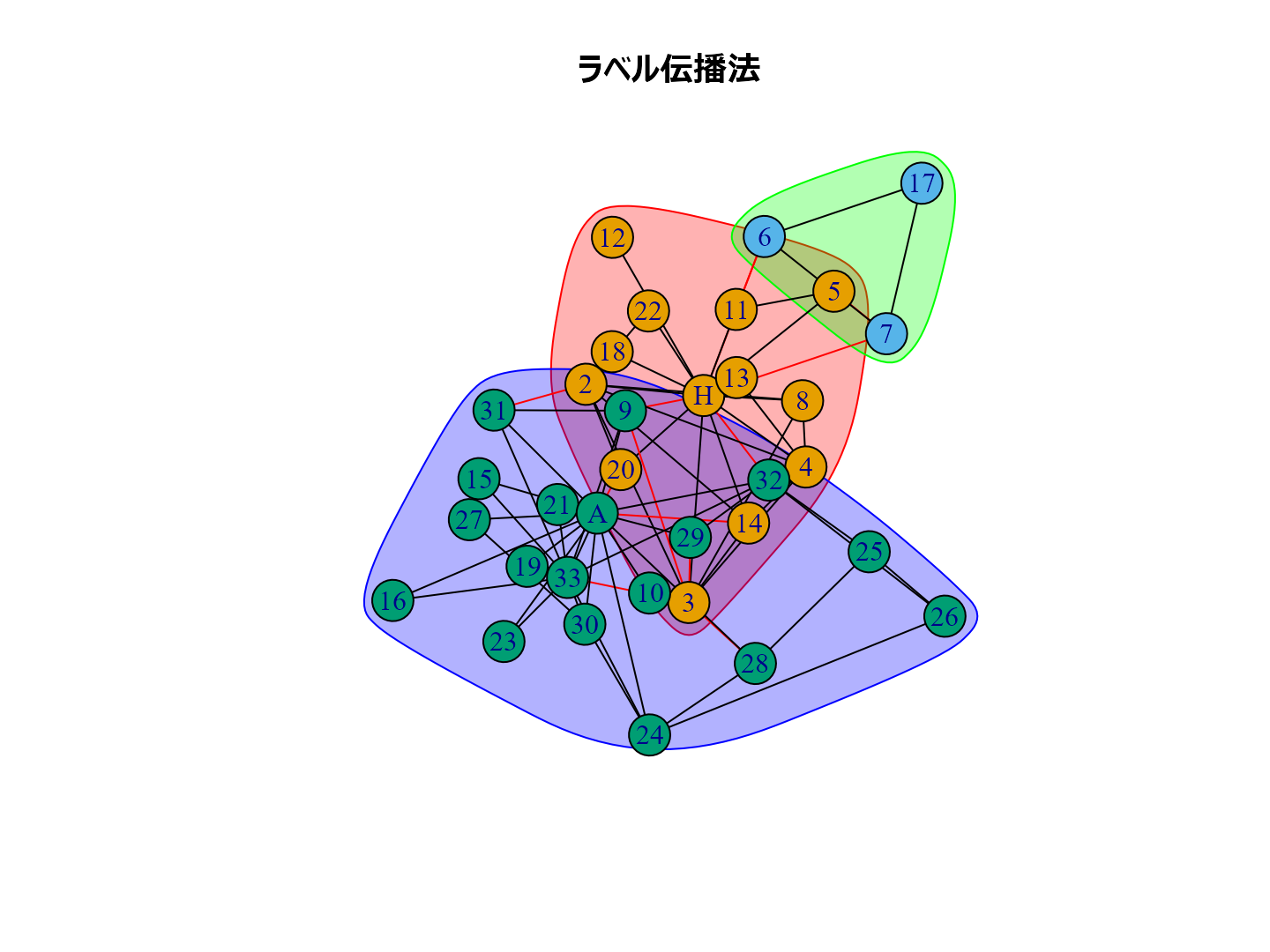


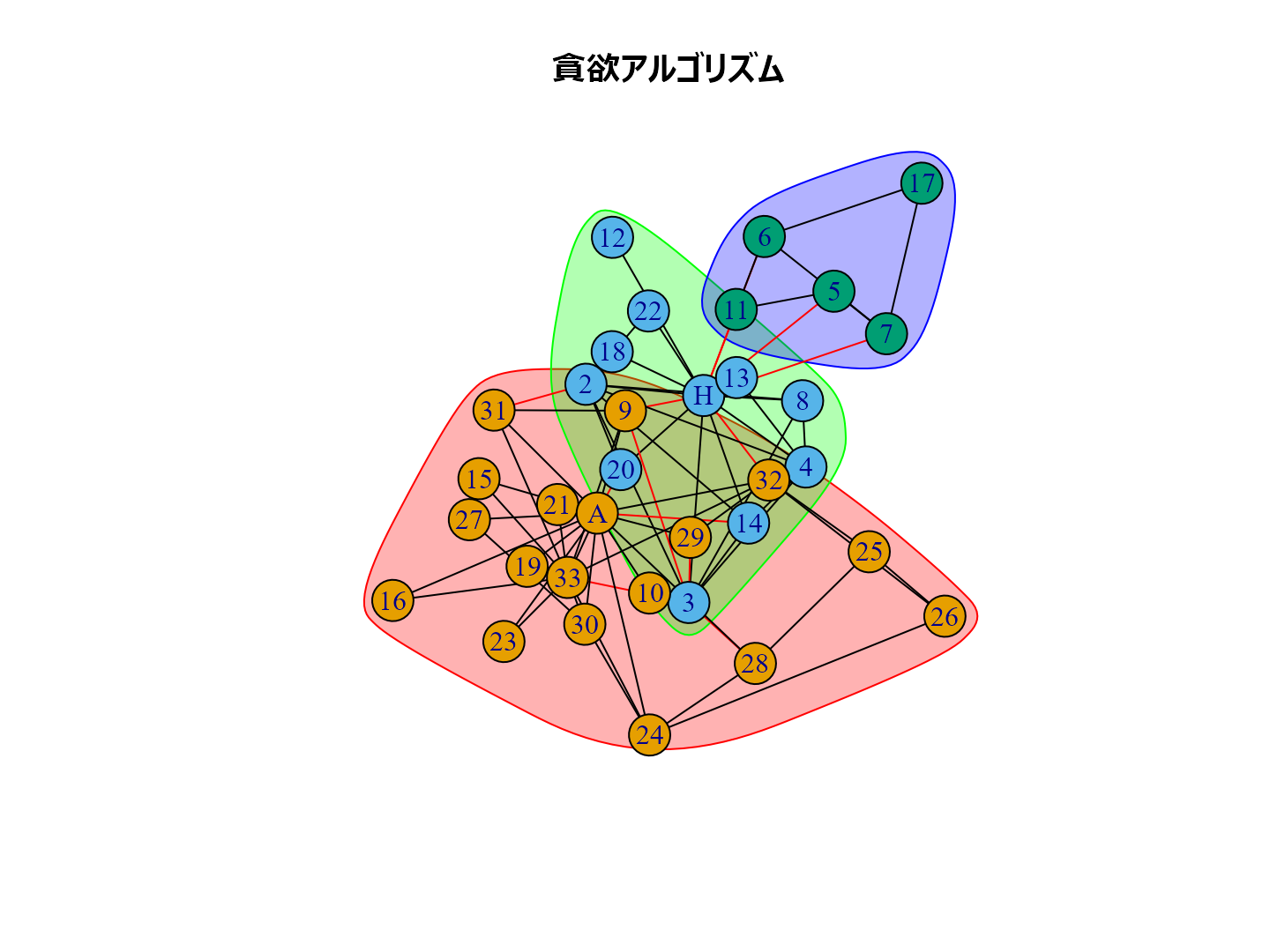


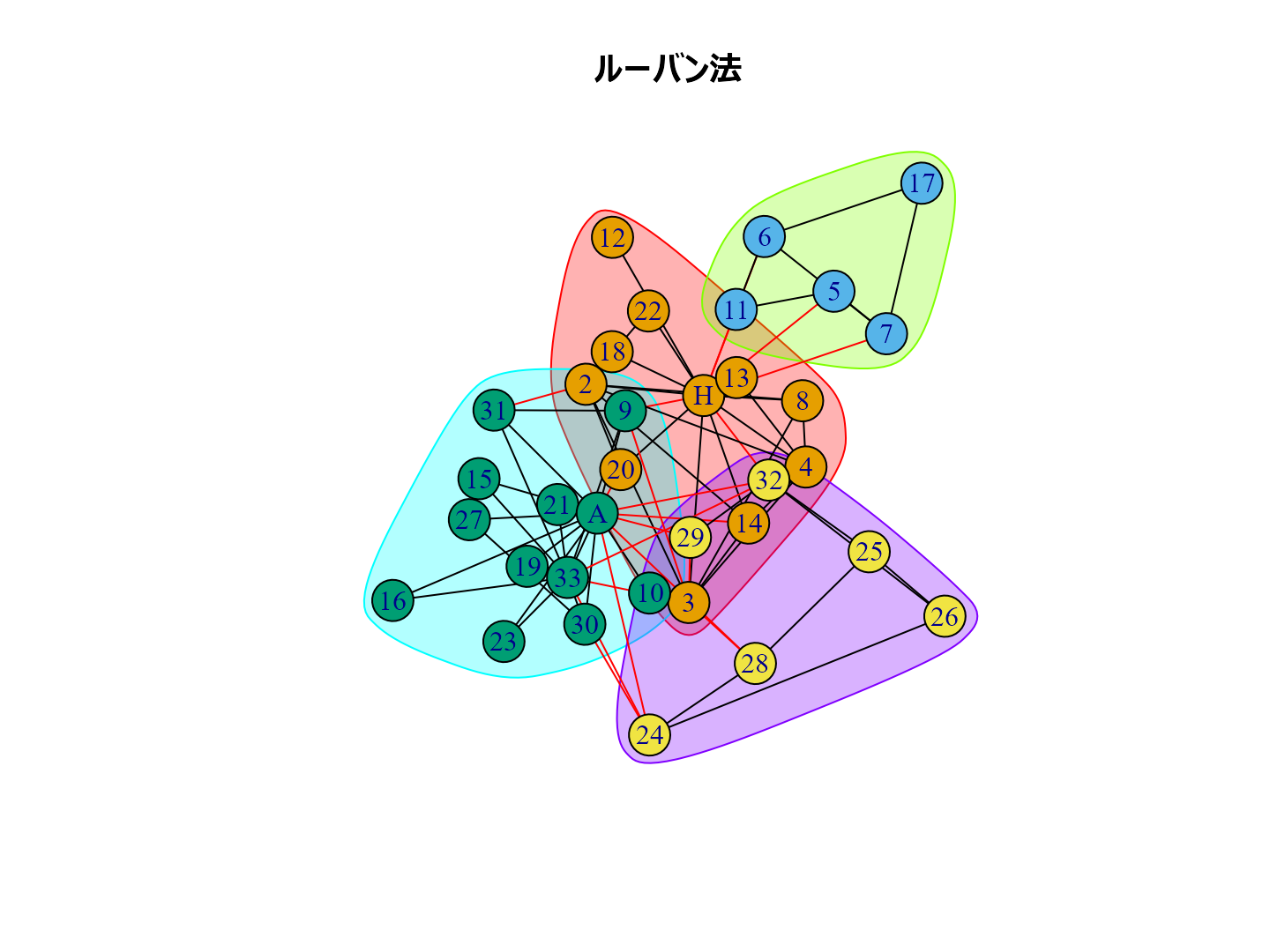
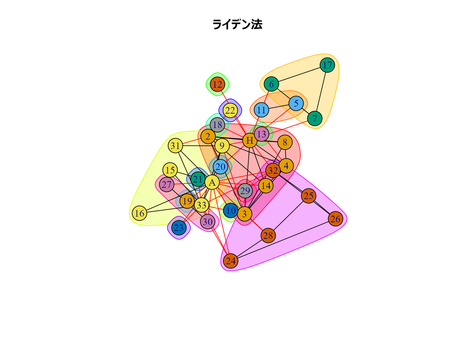
個人的な経験ではルーバン法がいい感じのグループ分けをしてくれるように思います。
Enjoy!
Rでサンタクロース
ふぉっふぉっふぉっ、みんな今年も良い子にしてたかな?
特にプレゼントはありません。
メリークリスマス!
library(conflicted)
library(tidyverse)
library(aplpack)
library(palmerpenguins)

pen_mean <- penguins |>
  select(bill_length_mm, bill_depth_mm, flipper_length_mm, body_mass_g, species, sex) |>
  drop_na() |>
  summarise(across(where(is.numeric), \(x) mean(x)), .by = c(species, sex)) |>
  arrange(species, sex)

faces(
  pen_mean |> select(bill_length_mm, bill_depth_mm, flipper_length_mm, body_mass_g),
  labels = paste0(pen_mean$species,"_",pen_mean$sex),
  fill = TRUE,
  face.type = 2,
  ncol.plot = 2,
  main = "南極パーマー基地のサンタクロースたち"
  )

qeMLパッケージの紹介
qeMLパッケージの紹介
先日開催された統計数理研究所ののR研究集会(共同研究集会「データ解析環境Rの整備と利用 」)で「qeMLパッケージの紹介」というLTをしてきました。
rjpusers.connpass.com
このパッケージを知ったきっかけはtjo氏のこのツイート。
{qeML}という"Quick & Easy wrapper for Machine Learning"を謳うRパッケージが出ているのをR-Bloggersを眺めていて知って、面白そう&便利そうなので入れてみようと思ったんだけど環境設定がコケてて入らない。誰か試した人います?https://t.co/eNwAJhntRs
— TJO (@TJO_datasci) 2023年11月27日
ちなみに研究会の現場で「Macでも動いたよ!」との証言がありました。
tidymodels、caret、mlr3、superlearner、SuperMLなどよりもはるかにシンプルなインターフェイスを持つ機械学習ラッパーです。
まだまだ未完成なのですが、非常に使い勝手が良さそうなので今後の発展に期待しています。
Enjoy!
『評価指標入門』をRで書く:多クラス分類の評価指標
『評価指標入門』をRで書く
この記事はR言語 Advent Calendar 2023 シリーズ2の16日目の記事です。
多クラス分類の評価指標
パッケージの呼び出し。
library(tidyverse)
library(palmerpenguins)
library(rsample)
library(yardstick)
library(ranger)
ペンギンの種類を判別するランダムフォレストのモデル。
pen_split <- penguins |>
  mutate(year = as.factor(year)) |>
  drop_na() |>
  initial_split(prop = 0.2, strata = species)

pen_train <- pen_split |>
  training()

pen_test <- pen_split |>
  testing()

fit_m_class <- pen_train |>
  ranger(species ~ ., data = _)

pred_test <- pen_test |>
  predict(fit_m_class, data = _)
以下の評価指標を算出
- 正解率(Accuracy)
- 適合率(Precision ; 精度)[macro, micro, weighted]
- 再現率(Recall, True Positive Rate ; TPR ; 感度)[macro, micro, weighted]
- F1-score[macro, micro, weighted]
# 正解率(Accuracy)
accuracy_vec(pen_test$species, pred_test$predictions)

# 適合率(Precision ; 精度)
precision_vec(pen_test$species, pred_test$predictions, estimator = "macro")
precision_vec(pen_test$species, pred_test$predictions, estimator = "micro")
precision_vec(pen_test$species, pred_test$predictions, estimator = "macro_weighted")

# 再現率(Recall, True Positive Rate ; TPR ; 感度)
recall_vec(pen_test$species, pred_test$predictions, estimator = "macro")
recall_vec(pen_test$species, pred_test$predictions, estimator = "micro")
recall_vec(pen_test$species, pred_test$predictions, estimator = "macro_weighted")

# F1-score
f_meas_vec(pen_test$species, pred_test$predictions, estimator = "macro")
f_meas_vec(pen_test$species, pred_test$predictions, estimator = "micro")
f_meas_vec(pen_test$species, pred_test$predictions, estimator = "macro_weighted")
ペンギンの種類の確率を推定するランダムフォレストのモデル。
fit_m_class_p <- pen_train |>
  ranger(species ~ ., data = _, probability = TRUE)

pred_test <- pen_test |>
  predict(fit_m_class_p, data = _)
ROC-AUCの算出
roc_auc_vec(pen_test$species, pred_test$predictions)
以上です。
『評価指標入門』をRで書く:二値分類における評価指標
『評価指標入門』をRで書く
この記事はR言語 Advent Calendar 2023 シリーズ2の13日目の記事です。
二値分類における評価指標
ライブラリーの呼び出し。
library(tidyverse)
library(palmerpenguins)
library(rsample)
library(MLmetrics)
library(yardstick)
library(pROC)
library(ranger)
ペンギンの性別を判別するランダムフォレストのモデル。
pen_split <- penguins |>
  mutate(year = as.factor(year)) |>
  drop_na() |>
  initial_split(prop = 0.2, strata = sex)

pen_train <- pen_split |>
  training()

pen_test <- pen_split |>
  testing()

fit_2_class <- pen_train |>
  ranger(sex ~ ., data = _)

pred_test <- pen_test |>
  predict(fit_2_class, data = _)
G-Meanのパッケージが見当たらなかったので実装する。
g_mean <- function (y_true, y_pred, positive = NULL)
{
  Confusion_DF <- ConfusionDF(y_pred, y_true)
  if (is.null(positive) == TRUE)
    positive <- as.character(Confusion_DF[1, 1])
  TP <- as.integer(subset(Confusion_DF, y_true == positive &
                            y_pred == positive)["Freq"])
  FN <- as.integer(sum(subset(Confusion_DF, y_true == positive &
                                y_pred != positive)["Freq"]))
  TN <- as.integer(subset(Confusion_DF, y_true != positive &
                            y_pred != positive)["Freq"])
  FP <- as.integer(sum(subset(Confusion_DF, y_true != positive &
                                y_pred == positive)["Freq"]))
  TPR <- TP/(TP + FN)
  TNR <- TN/(TP + FP)
  GM <- sqrt(TPR * TNR)
  return(GM)
}
以下の評価指標を算出。
- 正解率(Accuracy)
- マシューズ相関係数(Matthews Correlation coefficient ; MCC)
- 適合率(Precision ; 精度)
- 再現率(Recall, True Positive Rate ; TPR ; 感度)
- F1-score
- G-Mean(Geometric Mean)
Accuracy(pred_test$predictions, pen_test$sex)
mcc_vec(pred_test$predictions, pen_test$sex)
Precision(pred_test$predictions, pen_test$sex)
Recall(pred_test$predictions, pen_test$sex)
F1_Score(pred_test$predictions, pen_test$sex)
g_mean(pred_test$predictions, pen_test$sex)
ペンギンの性別の確率を推定するランダムフォレストのモデル。
fit_2_class_p <- pen_train |>
  mutate(sex = if_else(sex == "female", 1, 0)) |>
  ranger(sex ~ ., data = _)

pred_test <- pen_test |>
  mutate(sex = if_else(sex == "female", 1, 0)) |>
  predict(fit_2_class_p, data = _)
以下の評価指標を算出する。
- ROC-AUC(Receiver Operating Characteristic - Area Under the Curve)
- PR-AUC(Precision Recall - Area Under the Curve)
- pAUC(Partial Precision Area Under the Curve)
# ROC-AUC
AUC(
  pred_test$predictions,
  if_else(pen_test$sex == "female", 1, 0)
  )

# PR-AUC
PRAUC(
  pred_test$predictions,
  if_else(pen_test$sex == "female", 1, 0)
  )

# pAUC (α = 0, β = 0.2 の場合)
roc(
  if_else(pen_test$sex == "female", 1, 0),
  pred_test$predictions
  ) |>
  auc(partial.auc=c(0.0, 0.2), partial.auc.correct=TRUE)
以上です。
『評価指標入門』をRで書く:回帰の評価指標
『評価指標入門』をRで書く
この記事はR言語 Advent Calendar 2023 シリーズ2の12日目の記事です。
はじめに
2023年3月に出た『評価指標入門』という本がとても良かったのだけど、これまた公開されてるコードがPythonで。
いや、分かる。
分かるんだが。
分かるんだけど、やっぱりRで書きたいじゃん?
ということで、Rで書きます。
おことわり
- 解説は書きません。ぜひ書籍の方をお読みください。
- 特徴量エンジニアリングの部分はすっ飛ばして、評価指標の算出に絞っています。
- まちがいやより良い書き方があったらご指摘ください。
回帰の評価指標
パッケージの呼び出し。
library(tidyverse)
library(palmerpenguins)
library(rsample)
library(MLmetrics)
library(ranger)
ペンギンのデータで体重を目的変数にした回帰のランダムフォレストを例とします。
pen_split <- penguins |>
  mutate(year = as.factor(year)) |>
  drop_na() |>
  initial_split(prop = 0.2, strata = body_mass_g)

pen_train <- pen_split |>
  training()

pen_test <- pen_split |>
  testing()

fit_regression <- pen_train |>
  ranger(body_mass_g ~ ., data = _)

pred_test <- pen_test |>
  predict(fit_regression, data = _)
以下の評価指標を算出
- 平均絶対誤差(Mean Absolute Error ; MAE)
- 平均絶対パーセント誤差(Mean Absolute Percentage Error ; MAPE)
- 二乗平均平方誤差(Root Mean Squared Error ; RMSE)
- 対数平均二乗誤差(Root Mean Squared Log Error ; RMSLE)
- 平均二乗誤差(Mean Squared Error ; MSE)
- 決定係数
MAE(pred_test$predictions, pen_test$body_mass_g)
MAPE(pred_test$predictions, pen_test$body_mass_g)
RMSE(pred_test$predictions, pen_test$body_mass_g)
RMSLE(pred_test$predictions, pen_test$body_mass_g)
MSE(pred_test$predictions, pen_test$body_mass_g)
R2_Score(pred_test$predictions, pen_test$body_mass_g)
以上です。