『統計遺伝学』『遺伝統計学』の構成要素
sasLM
# SASというアプリの”analysis of variance according to the general linear model (PROC-GLM)"を実行してくれるパッケージ
# Rのパッケージ"sasLM"をインストールする

install.packages("sasLM")
# パッケージsasLMを使えるようにRの実行環境に読み込む
library(sasLM)
- パッケージには84検体のデータ CO2がある
> head(CO2)
  Plant   Type  Treatment conc uptake
1   Qn1 Quebec nonchilled   95   16.0
2   Qn1 Quebec nonchilled  175   30.4
3   Qn1 Quebec nonchilled  250   34.8
4   Qn1 Quebec nonchilled  350   37.2
5   Qn1 Quebec nonchilled  500   35.3
- 各サンプルには5つの情報がついている
- Plant
- Type
- Treatment
- conc
- uptake
- それぞれの中身を見てみる
- Plantは12種類が7サンプルずつ
- Typeの2群 QuebecとMississippiに1,2,3,1,2,3という番号が付与してあって、それにより、12種類
> table(CO2$Plant)

Qn1 Qn2 Qn3 Qc1 Qc3 Qc2 Mn3 Mn2 Mn1 Mc2 Mc3 Mc1
  7   7   7   7   7   7   7   7   7   7   7   7
-
- Typeは2群であることがわかる
> table(CO2$Type)

     Quebec Mississippi
         42          42
-
- Treatmentは2種類の介入方法、nonchilledとchilled
> table(CO2$Treatment)

nonchilled    chilled
        42         42
-
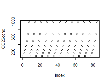
- concは実験「投与濃度」。異なる濃度を設定し、12種類のサンプルに7つずつの濃度で実験していることがわかる
plot(CO2$conc)
-
- uptakeは各サンプルで観測した、「知りたい値」の観測値。この値が、サンプルタイプ、処理タイプ(chiled or not)、concとどのような関係にあるかを調べたい
- 統計解析してみる
-
# このGLM()関数は、sasLMパッケージの関数
# CO2というデータフレームを使って
# uptakeがTypeとTreatmentとconcとを変数として線形回帰しているかどうかを調べる
# Type * Treatmentというのは、uptakeがTypeにも、Treatmentにも、TypeとTreatmentの組み合わせにも関係しているものとして線形回帰するつもりで解析する、という意味
# uptake = a1 Type + a2 Treatment + a3 (Type * Treatmen) + a4 conc + 乱雑項
# という式に当てはめて、よい感じのa1,a2,a3,a4を推定する
# そのうえで、その推定したa1,a2,a3,a4が本当に信じてよいかどうかをp値にして評価する
# その「統計学的検定手法」がANOVA
# p値が小さければa1,a2,a3,a4のそれぞれがを信じてよいと考える

GLM(uptake ~ Type*Treatment + conc, Data=CO2, lsm=TRUE)
# 出力
> GLM(uptake ~ Type*Treatment + conc, Data=CO2, lsm=TRUE)
# Pr(>F)がp値のこと。とても小さいので、線形回帰したモデルを全体として信じてよいということ
$ANOVA
Response : uptake
                Df Sum Sq Mean Sq F value    Pr(>F)
MODEL            4 6864.4 1716.09  47.693 < 2.2e-16 ***
RESIDUALS       79 2842.6   35.98
CORRECTED TOTAL 83 9707.0
---
Signif. codes:  0 ‘***’ 0.001 ‘**’ 0.01 ‘*’ 0.05 ‘.’ 0.1 ‘ ’ 1

# 調べた4つの項、Type, Treatment, TypeとTreatmentの組み合わせ項、concのすべてについてPr(>F) (p値のこと)が小さいので、すべての項目をそれぞれ信じてよいということ
# Type I , Type II, Type III というのは、一種の流儀の違いだが、ここではどれも同じ値を返しているので、区別を気にしなくてよい
$`Type I`
               Df Sum Sq Mean Sq F value    Pr(>F)
Type            1 3365.5  3365.5 93.5330 4.774e-15 ***
Treatment       1  988.1   988.1 27.4611 1.300e-06 ***
Type:Treatment  1  225.7   225.7  6.2733   0.01432 *
conc            1 2285.0  2285.0 63.5032 1.002e-11 ***
---
Signif. codes:  0 ‘***’ 0.001 ‘**’ 0.01 ‘*’ 0.05 ‘.’ 0.1 ‘ ’ 1

$`Type II`
               Df Sum Sq Mean Sq F value    Pr(>F)
Type            1 3365.5  3365.5 93.5330 4.774e-15 ***
Treatment       1  988.1   988.1 27.4611 1.300e-06 ***
Type:Treatment  1  225.7   225.7  6.2733   0.01432 *
conc            1 2285.0  2285.0 63.5032 1.002e-11 ***
---
Signif. codes:  0 ‘***’ 0.001 ‘**’ 0.01 ‘*’ 0.05 ‘.’ 0.1 ‘ ’ 1

$`Type III`
               Df Sum Sq Mean Sq F value    Pr(>F)
Type            1 3365.5  3365.5 93.5330 4.774e-15 ***
Treatment       1  988.1   988.1 27.4611 1.300e-06 ***
Type:Treatment  1  225.7   225.7  6.2733   0.01432 *
conc            1 2285.0  2285.0 63.5032 1.002e-11 ***
---
Signif. codes:  0 ‘***’ 0.001 ‘**’ 0.01 ‘*’ 0.05 ‘.’ 0.1 ‘ ’ 1

# ここは、「検定」の結果として、「信じてよい」ということが分かったので
# 以下の「推定」結果を信じましょう、その「推定結果a1,a2,a3,a4はこのくらいの値ですよ」という推定結果
# TypeがQuebecだと、Quebecの数が1,2,3と変わると、1増えるごとに、9.3810だけ、uptakeの値が大きくなる傾向があるよ、TypeがMississippiだとuptakeは増えないよ、という意味。
# nonchilledとchilledではnonchilledなら10.1381だけuptakeが増えるが、chilledだと増えないという意味
$Parameter
                                    Estimate Estimable Std. Error Df
(Intercept)                           8.1015         0    1.62794 79
TypeQuebec                            9.3810         0    1.85119 79
TypeMississippi                       0.0000         0    0.00000 79
Treatmentnonchilled                  10.1381         0    1.85119 79
Treatmentchilled                      0.0000         0    0.00000 79
TypeQuebec:Treatmentchilled           6.5571         0    2.61797 79
TypeQuebec:Treatmentnonchilled        0.0000         0    0.00000 79
TypeMississippi:Treatmentchilled      0.0000         0    0.00000 79
TypeMississippi:Treatmentnonchilled   0.0000         0    0.00000 79
conc                                  0.0177         1    0.00222 79
                                    t value  Pr(>|t|)
(Intercept)                          4.9765 3.709e-06 ***
TypeQuebec                           5.0675 2.590e-06 ***
TypeMississippi
Treatmentnonchilled                  5.4765 4.988e-07 ***
Treatmentchilled
TypeQuebec:Treatmentchilled          2.5047   0.01432 *
TypeQuebec:Treatmentnonchilled
TypeMississippi:Treatmentchilled
TypeMississippi:Treatmentnonchilled
conc                                 7.9689 1.002e-11 ***
---
Signif. codes:  0 ‘***’ 0.001 ‘**’ 0.01 ‘*’ 0.05 ‘.’ 0.1 ‘ ’ 1

$`Least Square Mean`
                                      LSmean  LowerCL  UpperCL        SE
(Intercept)                         27.21310 25.91036 28.51583 0.6544929
TypeQuebec                          33.54286 31.70051 35.38520 0.9255927
TypeMississippi                     20.88333 19.04099 22.72568 0.9255927
Treatmentnonchilled                 30.64286 28.80051 32.48520 0.9255927
Treatmentchilled                    23.78333 21.94099 25.62568 0.9255927
conc                                27.21310 25.91036 28.51583 0.6544929
TypeQuebec:Treatmentchilled         31.75238 29.14691 34.35785 1.3089858
TypeQuebec:Treatmentnonchilled      35.33333 32.72786 37.93880 1.3089858
TypeMississippi:Treatmentchilled    15.81429 13.20881 18.41976 1.3089858
TypeMississippi:Treatmentnonchilled 25.95238 23.34691 28.55785 1.3089858
                                    Df
(Intercept)                         79
TypeQuebec                          79
TypeMississippi                     79
Treatmentnonchilled                 79
Treatmentchilled                    79
conc                                79
TypeQuebec:Treatmentchilled         79
TypeQuebec:Treatmentnonchilled      79
TypeMississippi:Treatmentchilled    79
TypeMississippi:Treatmentnonchilled 79

> GLM(uptake ~ Type*Treatment + conc, Data=CO2, lsm=TRUE)
$ANOVA
Response : uptake
                Df Sum Sq Mean Sq F value    Pr(>F)
MODEL            4 6864.4 1716.09  47.693 < 2.2e-16 ***
RESIDUALS       79 2842.6   35.98
CORRECTED TOTAL 83 9707.0
---
Signif. codes:  0 ‘***’ 0.001 ‘**’ 0.01 ‘*’ 0.05 ‘.’ 0.1 ‘ ’ 1

$`Type I`
               Df Sum Sq Mean Sq F value    Pr(>F)
Type            1 3365.5  3365.5 93.5330 4.774e-15 ***
Treatment       1  988.1   988.1 27.4611 1.300e-06 ***
Type:Treatment  1  225.7   225.7  6.2733   0.01432 *
conc            1 2285.0  2285.0 63.5032 1.002e-11 ***
---
Signif. codes:  0 ‘***’ 0.001 ‘**’ 0.01 ‘*’ 0.05 ‘.’ 0.1 ‘ ’ 1

$`Type II`
               Df Sum Sq Mean Sq F value    Pr(>F)
Type            1 3365.5  3365.5 93.5330 4.774e-15 ***
Treatment       1  988.1   988.1 27.4611 1.300e-06 ***
Type:Treatment  1  225.7   225.7  6.2733   0.01432 *
conc            1 2285.0  2285.0 63.5032 1.002e-11 ***
---
Signif. codes:  0 ‘***’ 0.001 ‘**’ 0.01 ‘*’ 0.05 ‘.’ 0.1 ‘ ’ 1

$`Type III`
               Df Sum Sq Mean Sq F value    Pr(>F)
Type            1 3365.5  3365.5 93.5330 4.774e-15 ***
Treatment       1  988.1   988.1 27.4611 1.300e-06 ***
Type:Treatment  1  225.7   225.7  6.2733   0.01432 *
conc            1 2285.0  2285.0 63.5032 1.002e-11 ***
---
Signif. codes:  0 ‘***’ 0.001 ‘**’ 0.01 ‘*’ 0.05 ‘.’ 0.1 ‘ ’ 1

$Parameter
                                    Estimate Estimable Std. Error Df
(Intercept)                           8.1015         0    1.62794 79
TypeQuebec                            9.3810         0    1.85119 79
TypeMississippi                       0.0000         0    0.00000 79
Treatmentnonchilled                  10.1381         0    1.85119 79
Treatmentchilled                      0.0000         0    0.00000 79
TypeQuebec:Treatmentchilled           6.5571         0    2.61797 79
TypeQuebec:Treatmentnonchilled        0.0000         0    0.00000 79
TypeMississippi:Treatmentchilled      0.0000         0    0.00000 79
TypeMississippi:Treatmentnonchilled   0.0000         0    0.00000 79
conc                                  0.0177         1    0.00222 79
                                    t value  Pr(>|t|)
(Intercept)                          4.9765 3.709e-06 ***
TypeQuebec                           5.0675 2.590e-06 ***
TypeMississippi
Treatmentnonchilled                  5.4765 4.988e-07 ***
Treatmentchilled
TypeQuebec:Treatmentchilled          2.5047   0.01432 *
TypeQuebec:Treatmentnonchilled
TypeMississippi:Treatmentchilled
TypeMississippi:Treatmentnonchilled
conc                                 7.9689 1.002e-11 ***
---
Signif. codes:  0 ‘***’ 0.001 ‘**’ 0.01 ‘*’ 0.05 ‘.’ 0.1 ‘ ’ 1

$`Least Square Mean`
                                      LSmean  LowerCL  UpperCL        SE
(Intercept)                         27.21310 25.91036 28.51583 0.6544929
TypeQuebec                          33.54286 31.70051 35.38520 0.9255927
TypeMississippi                     20.88333 19.04099 22.72568 0.9255927
Treatmentnonchilled                 30.64286 28.80051 32.48520 0.9255927
Treatmentchilled                    23.78333 21.94099 25.62568 0.9255927
conc                                27.21310 25.91036 28.51583 0.6544929
TypeQuebec:Treatmentchilled         31.75238 29.14691 34.35785 1.3089858
TypeQuebec:Treatmentnonchilled      35.33333 32.72786 37.93880 1.3089858
TypeMississippi:Treatmentchilled    15.81429 13.20881 18.41976 1.3089858
TypeMississippi:Treatmentnonchilled 25.95238 23.34691 28.55785 1.3089858
                                    Df
(Intercept)                         79
TypeQuebec                          79
TypeMississippi                     79
Treatmentnonchilled                 79
Treatmentchilled                    79
conc                                79
TypeQuebec:Treatmentchilled         79
TypeQuebec:Treatmentnonchilled      79
TypeMississippi:Treatmentchilled    79
TypeMississippi:Treatmentnonchilled 79
証拠としての立場からのAIアシスト for 医療画像・病理
- 資料
www.nature.com
www.nature.com
diagnosticpathology.biomedcentral.com
https://digitalpathologyassociation.org/_data/cms_files/files/PathologyAI_ReferencGuide.pdf
Use of advanced artificial intelligence in forensic medicine
A narrative review of digital pathology and artificial intelligence: focusing on lung cancer - Sakamoto - Translational Lung Cancer Research
research.adobe.com
*-演算、*-代数、量子確率論、量子力学、作用素、非可換作用素、不確定性原理、作用素環、非可換幾何
- いくつかの資料
- 多元環は、ベクトルとか行列とか
- そこに*-演算を入れる。複素数でうまく行く演算
- 多元環に*-演算を持たせると、*-代数
- *-代数の中にC*-代数とかがある
- 量子確率論は、*-代数 A と、状態のペア
とされる。古典確率論が
のトリオとされるのに対応する
は確率変数となって、そのモーメント列が決まるという意味で、確率変数を決定する
- ただし、モーメント列というとき、古典確率変数の場合は1,2,3,...次モーメントが決まるわけだが、量子確率変数の場合は、
のように、確率変数のk乗の概念が、
と
との並べ方で代わって来るので複雑化する
- なお、この「状態」というのは、
なる写像のこと
- 状態の例としては、確率変数a が行列表現を持っているときに、そのトレース/次元を返すものや、あるベクトル
があったときに
として得られるものなどがある
- 状態の例としては、確率変数a が行列表現を持っているときに、そのトレース/次元を返すものや、あるベクトル
- 一方、量子力学で物理量が作用素である、というのは、物理量の期待値が
として得られる、という意味
- 他方、物理量が行列の形をしているということは、
である(ことが一般的である)。このようなとき、「
とは同時固有値を持ちえない」という話があるらしい、この同時に固有値が持てないから、同時に測定ができないということ(らしい)
- スペクトルというのは、モーメント列に相当する(らしい)。したがって可換作用素のスペクトルというのは固有値と関連して定まって来る
- 非可換作用素のスペクトルはモーメント列の意味が変わって来るが、そのあたりをいじることで、非可換作用素同士の「環構造」を考えて、その構造を幾何で考えると非可換幾何
ぱらぱらめくる『An Introductory Course on Non-commutative Information Geometry』
- PDF:An Introductory Course on Non-commutative Information Geometry・・・めくるには体力がまだ不足しているので、『めくる前』の整理をすることにする
- ぱらぱらめくる前に。動機
- 数の概念の拡張として作用を考える(演算子・作用素というパラダイム)
- 数の概念を拡張していくと、複素数が登場し、大小比較ができなくなる。さらに行列を考えると、積の可換性が失われる。そういう意味で行列は拡張された数
- 同様に、関数を、ある値(のセット)を取って、ある値を返すものとしたとき、関数を足したり、係数倍したりできるので、関数自体も、数らしさを持つ(関数+関数=関数、係数x関数=関数)。この観点で関数を数の拡張とみなす
- いずれにしても、数も数の拡張としての行列も関数も、抽象的なベクトル空間の点とみなせるし、行列の集まり・関数の集まりがベクトル空間として扱える
- ある性質を持った関数の集まりが環をなしているとき、その関数の環は空間(多様体)のように見える。関数の環を考えることと、対応する空間を考えることは同じことになる。ここで考えている関数は積に関して可換なので、対応する空間も可換性を持った空間になっている
- 作用素というのは、ベクトル空間の点を取って値を返すものでる。作用素(演算子とも言う。英語でoperator)は量子論での物理量に相当するように、古典物理学では「ある値を持つもの」という意味で「数」だったが、量子論では「作用素」であり、「行列・テンソル」の形をしている。また、線形作用素を考えるとき、線形汎関数Wikipedia)として作用素を見ることもできる。このように作用素を考えると行列演算子的に見える。行列なので積が非可換
- 他方、作用素を、「点」を取って「値」を返すと考えると関数に見える
- 結局、作用素は行列的な数の拡張でもあり、関数的な数の拡張でもある
- 関数的に拡張したと考えれば、(可換性を持った)空間に対応づくし、行列的に拡張したと考えれば、非可換性を持つ
- 両方の性質を持つ作用素には、非可換性を持った空間に対応しそうである
- さて。情報幾何では関数が多様体になっているとともに、KL-divergenceが非対称である。非可換性を持った空間を考えることと相通じる感じがする
- ということで、非可換作用素環とその空間を情報幾何とつなげるとどうなるのかを考えることは興味深い
- 以上が、この『ぱらぱらめくる』シリーズの動機
- 数の概念の拡張として作用を考える(演算子・作用素というパラダイム)
- 『ぱらぱらめくる』前に基礎事項の確認
Metropolis Hastings サンプリングする
# 値の台
xx <- seq(from=-5,to=20,length=1000)

# 適当な(密度関数)
dd <- dnorm(xx) + dnorm(xx,1,2) + dnorm(xx,10,2)

# 確率密度関数っぽい形
plot(xx,dd)

#
library(mcmc)

# 確率密度に比例したあたいの対数を返す関数を書く
h <- function(x){
	log(dnorm(x) + dnorm(x,1,2) + dnorm(x,10,2))
}
# サンプリングする
# 2番目の引数は、始めに試す乱数の値
#
out <- metrop(h, 0, 10000)
out$accept

# out[[2]]には試した値が格納される
# out$accept.batchには、0/1が格納され、採択されたものには1が立つのでそれを選ぶ

hist(out[[2]][which(out$accept.batch==1)])