The Nix daemon uses a custom binary protocol — the nix daemon protocol — to
communicate with just about everything. When you run nix build on your
machine, the Nix binary opens up a Unix socket to the Nix daemon and talks
to it using the Nix protocol1. When you administer a Nix server remotely using
nix build --store ssh-ng://example.com [...], the Nix binary opens up an SSH
connection to a remote machine and tunnels the Nix protocol over SSH. When you
use remote builders to speed up your Nix builds, the local and remote Nix daemons speak
the Nix protocol to one another.
Despite its importance in the Nix world, the Nix protocol has no specification
or reference documentation. Besides the original implementation in the Nix
project itself, the hnix-store project contains a re-implementation of the
client end of the protocol. The gorgon project contains a partial re-implementation
of the protocol in Rust, but we didn’t know about it when we started. We do not know of any other implementations. (The
Tvix project created its own gRPC-based
protocol instead of re-implementing a Nix-compatible one.)
So we re-implemented the Nix protocol, in Rust.
We started it mainly as a learning exercise, but we’re hoping to do some useful things along the way:
Document and demystify the protocol. (That’s why we wrote this blog post! 👋)
Enable new kinds of debugging and observability. (We tested our implementation with a little Nix proxy
that transparently forwards the Nix protocol while also writing a log.)
Empower other third-party Nix clients and servers. (We wrote an
experimental tool that acts as a Nix remote builder, but proxies the
actual build over the Bazel Remote Execution protocol.)
Unlike the hnix-store re-implementation, we’ve implemented both ends of the protocol.
This was really helpful for testing, because it allowed our debugging proxy to verify
that a serialization/deserialization round-trip gave us something
byte-for-byte identical to the original. And thanks
to Rust’s procedural macros and the serde crate, our implementation is
declarative, meaning that it also serves as concise documentation of the
protocol.
Structure of the Nix protocol
A Nix communication starts with the exchange of a few magic bytes, followed by
some version negotiation. Both the client and server maintain compatibility with
older versions of the protocol, and they always agree to speak the newest version
supported by both.
The main protocol loop is initiated by the client, which sends a “worker op� consisting
of an opcode and some data. The server gets to work on carrying out the requested operation.
While it does so, it enters a “stderr streaming� mode in which it sends a stream of
logging or tracing messages back to the client (which is how Nix’s progress messages
make their way to your terminal when you run a nix build). The stream of stderr messages
is terminated by a special STDERR_LAST message. After that, the server sends the operation’s
result back to the client (if there is one), and waits for the next worker op to come along.
The Nix wire format
Nix’s wire format starts out simple. It has two basic types:
unsigned 64-bit integers, encoded in little-endian order; and
byte buffers, written as a length (a 64-bit integer) followed by the bytes in the buffer.
If the length of the buffer is not a multiple of 8, it is zero-padded to a multiple of 8 bytes.
Strings on the wire are just byte buffers, with no specific encoding.
Compound types are built up in terms of these two pieces:
Variable-length collections like lists, sets, or maps are represented by the number of elements they contain (as a 64-bit integer) followed by their contents.
Product types (i.e. structs) are represented by listing out their fields one-by-one.
Sum types (i.e. unions) are serialized with a tag followed by the contents.
For example, a “valid path info� consists of a deriver (a byte buffer), a hash (a byte buffer),
a set of references (a sequence of byte buffers), a registration time (an integer), a nar size (an integer),
a boolean (represented as an integer in the protocol), a set of signatures (a sequence of byte buffers), and
finally a content address (a byte buffer). On the wire, it looks like:
This wire format is not self-describing: in order to read it, you need
to know in advance which data-type you’re expecting. If you get confused or misaligned somehow,
you’ll end up reading complete garbage. In my experience, this usually leads to
reading a “length� field that isn’t actually a length, followed by an attempt to allocate
exabytes of memory. For example, suppose we were trying to read the “valid path info� written
above, but we were expecting it to be a “valid path info with path,� which is the same as a
valid path info except that it has an extra path at the beginning. We’d misinterpret
/nix/store/c3f-...-hello-2.12.1.drv as the path, we’d misinterpret the hash as the
deriver, we’d misinterpret the number of references (2) as the number of bytes in
the hash, and we’d misinterpret the length of the first reference as the hash’s data.
Finally, we’d interpret /nix/sto as a 64-bit integer and promptly crash as we
allocate space for more than <semantics>8×10¹⁸<annotation encoding="application/x-tex">8 \times 10^{18}</annotation></semantics>8×1018 references.
There’s one important exception to the main wire format: “framed data�.
Some worker ops need to transfer source trees or build artifacts that are too
large to comfortably fit in memory; these large chunks of data need to be
handled differently than the rest of the protocol. Specifically, they’re transmitted
as a sequence of length-delimited byte buffers, the idea being that you can read one
buffer at a time, and stream it back out or write it to disk before reading the next
one.
Two features make this framed data unusual:
the sequence of buffers are terminated by an empty buffer instead of being length-delimited
like most of the protocol, and the individual buffers are not padded out to a multiple of 8 bytes.
Serde
Serde is the de-facto standard for serialization and deserialization in Rust. It
defines an interface between serialization formats (like JSON, or the Nix wire
protocol) on the one hand and serializable data types on the other. This divides our
work into two parts: first, we implement the serialization format, by specifying the
correspondence between Serde’s data model and the Nix wire format we described above.
Then we describe how the Nix protocol’s messages map to the Serde data model.
The best part about using Serde for this task is that the second step becomes
straightforward and completely declarative. For example, the AddToStore worker op
is implemented like
These few lines handle both serialization and deserialization of the AddToStore worker op,
while ensuring that they remain in-sync.
Mismatches with the Serde data model
While Serde gives us some useful tools and shortcuts, it isn’t a perfect fit for our case.
For a start, we don’t benefit much from one of Serde’s most important benefits: the decoupling
between serialization formats and serializable data types. We’re interested in a specific
serialization format (the Nix wire format) and a specific collection of data types (the ones
used in the Nix protocol); we don’t gain much by being able to, say,
serialize the Nix protocol to JSON.
The main disadvantage of using Serde is that we need to match the Nix protocol to Serde’s data
model. Most things match fairly well; Serde has native support for integers, byte buffers,
sequences, and structs. But there were a few mismatches that we had to work around:
Different kinds of sequences: Serde has native support for sequences, and it can support
sequences that are either length-delimited or not. However, Serde does not make it easy to support
length-delimited and non-length-delimited sequences in the same serialization format. And
although most sequences in the Nix format are length-delimited, the sequence of chunks in a
framed source are not. We hacked around this restriction by treating a framed source not
as a sequence but as a tuple with <semantics>264<annotation encoding="application/x-tex">2^{64}</annotation></semantics>264 elements, relying on the fact that Serde doesn’t care
if you terminate a tuple early.
The Serde data model is larger than the Nix protocol needs; for example, it supports floating
point numbers, and integers of different sizes and signedness. Our Serde de/serializer raises
an error at runtime if it encounters any of these data types. Our Nix protocol implementation
avoids these forbidden data types, but the Serde abstraction between the serializer and the
data types means that any mistakes will not be caught at compile time.
Sum types tagged with integers: Serde has native support for tagged unions, but it assumes
that they’re tagged with either the variant name (i.e. a string) or the variant’s index within
a list of all possible variants. The Nix protocol uses numeric tags, but we can’t just
use the variant’s index: we need to specify specific tags for specific variants, to match the
ones used by Nix. We solved this by using our own derive macro for tagged unions. Instead of
using Serde’s native unions, we map a union to a Serde tuple consisting of a tag followed by
its payload.
But with these mismatches resolved, our final definition of the Nix protocol is fully declarative
and pretty straightforward:
#[derive(TaggedSerde)]// ^^ our custom procedural macro for unions tagged with integerspubenumWorkerOp{#[tagged_serde = 1]// ^^ this op has opcode 1IsValidPath(StorePath,Resp<bool>),// ^^ ^^ the op's response type// || the op's payload#[tagged_serde = 6]QueryReferrers(StorePath,Resp<StorePathSet>),#[tagged_serde = 7]AddToStore(AddToStore,Resp<ValidPathInfoWithPath>),#[tagged_serde = 9]BuildPaths(BuildPaths,Resp<u64>),#[tagged_serde = 10]EnsurePath(StorePath,Resp<u64>),#[tagged_serde = 11]AddTempRoot(StorePath,Resp<u64>),#[tagged_serde = 14]FindRoots((),Resp<FindRootsResponse>),// ... another dozen or so ops}
Next steps
Our implementation is still a work in progress; most notably the API needs a lot
of polish. It also only supports protocol version 34, meaning it cannot interact
with old Nix implementations (before 2.8.0, which was released in 2022) and will lack support for features
introduced in newer versions of the protocol.
Since in its current state our Nix protocol implementation can
already do some useful things, we’ve made the crate available on crates.io.
If you have a use-case that isn’t supported yet, let us know! We’re still trying to figure
out what can be done with this.
In the meantime, now that we can handle the Nix remote protocol itself we’ve shifted our
experimental hacking over to integrating with Bazel remote execution.
We’re writing a program that presents itself as a Nix remote builder, but instead of executing
the builds itself it sends them via the Bazel Remote Execution API to some other build
infrastructure. And then when the build is done, our program sends it back to the requester as though
it were just a normal Nix remote builder.
But that’s just our plan, and we think there must be more applications of this. If you could speak
the Nix remote protocol, what would you do with it?
ghc-debug is a debugging tool for performing precise heap analysis of Haskell programs
(check out our previous post introducing it).
While working on Eras Profiling, we took the opportunity to make some much
needed improvements and quality of life fixes to both the ghc-debug library and the
ghc-debug-brick terminal user interface.
To summarise,
ghc-debug now works seamlessly with profiled executables.
The ghc-debug-brick UI has been redesigned around a composable, filter based workflow.
Cost centers and other profiling metadata can now be inspected using both the library
interface and the TUI.
More analysis modes have been integrated into the terminal interface such as
the 2-level profile.
This post explores the changes and the new possibilities for inspecting
the heap of Haskell processes that they enable. These changes are available
by using the 0.6.0.0 version of ghc-debug-stub and ghc-debug-brick.
Recap: using ghc-debug
There are typically two processes involved when using ghc-debug on a live program.
The first is the debuggee process, which is the process whose heap you want to inspect.
The debuggee process is linked against the ghc-debug-stub package. The ghc-debug-stub
package provides a wrapper function
withGhcDebug ::IO a ->IO a
that you wrap around your main function to enable the use of ghc-debug. This wrapper
opens a unix socket and answers queries about the debuggee process’ heap, including
transmitting various metadata about the debuggee, like the ghc version it was compiled with,
and the actual bits that make up various objects on the heap.
The second is the debugger process, which queries the debuggee via the socket
mechanism and decodes the responses to reconstruct a view of the debuggee’s
Haskell heap. The most common debugger which people use is ghc-debug-brick, which
provides a TUI for interacting with the debuggee process.
It is an important principle of ghc-debug that the debugger and debuggee don’t
need to be compiled with the same version of GHC as each other. In other words,
a debugger compiled once is flexible to work with many different debuggees. With
our most recent changes debuggers now work seamlessly with profiled executables.
TUI improvements
Exploring Cost Center Stacks in the TUI
For debugging profiled executables, we added support for decoding
profiling information in the ghc-debug library. Once decoding support was added, it’s easy to display the
associated cost center stack information for each closure in the TUI, allowing you to
interactively explore that chain of cost
centers with source locations that lead to a particular closure being allocated.
This gives you the same information as calling the GHC.Stack.whoCreated function
on a closure, but for every closure on the heap!
Additionally, ghc-debug-brick allows you to search for closures that have been
allocated under a specific cost center.
If other profiling modes like retainer profiling or biographical profiling are enabled,
then the extra word tracked by those modes is used to mark used closures with a green line.
Typical ghc-debug-brick workflows would involve connecting to the client process
or a snapshot and then running queries like searches to track down the objects that
you are interested in. This took the form of various search commands available in the
UI:
However, sometimes you would like to combine multiple search commands, in order to
more precisely narrow down the exact objects you are interested in. Earlier you
would have to do this by either writing custom queries with the ghc-debug Haskell
API or modify the ghc-debug-brick code itself to support your custom queries.
Filters provide a composable workflow in order to perform more advanced queries.
You can select a filter to apply from a list of possible filters, like the
constructor name, closure size, era etc. and add it to the current filter stack
to make custom search queries. Each filter can also be inverted.
We were motivated to add this feature after implementing support for eras profiling
as it was often useful to combine existing queries with a filter by era.
With these filters it’s easy to express your own domain specific queries, for example:
Find the Foo constructors which were allocated in a certain era.
Find all ARR_WORDS closures which are bigger than 1000 bytes.
Show me everything retained in this era, apart from ARR_WORDS and GRE constructors.
Here is a complete list of filters which are currently available:
Name
Input
Example
Action
Address
Closure Address
0x421c3d93c0
Find the closure with the specific address
Info Table
Info table address
0x1664ad70
Find all closures with the specific info table
Constructor Name
Constructor name
Bin
Find all closures with the given constructor name
Closure Name
Name of closure
sat_sHuJ_info
Find all closures with the specific closure name
Era
<era>/<start-era>-<end-era>
13 or 9-12
Find all closures allocated in the given era range
Cost centre ID
A cost centre ID
107600
Finds all closures allocated (directly or indirectly) under this cost centre ID
Closure Size
Int
1000
Find all closures larger than a certain size
Closure Type
A closure type description
ARR_WORDS
Find all ARR_WORDS closures
All these queries are retainer queries which will not only show you the closures
in question but also the retainer stack which explains why they are retained.
Improvements to profiling commands
ghc-debug-brick has long provided a profile command which performs a heap
traversal and provides a summary like a single sample from a -hT profile.
The result of this query is now displayed interactively in the terminal interface.
For each entry, the left column in the header shows the type of closure in
question, the total number of this closure type which are allocated,
the number of bytes on the heap taken up by this closure, the maximum size of each of
these closures and the average size of each allocated closure.
The right column shows the same statistics, but taken over all closures in the
current heap sample.
Each entry can be expanded, five sample points from each band are saved so you can
inspect some closures which contributed to the size of the band. For example, here we
expand the THUNK closure and can see a sample of 5 thunks which contribute to the 210,000
thunks which are live on this heap.
Support for the 2-level closure type profile has also been added to the TUI.
The 2-level profile is more fine-grained than the 1-level profile as the profile
key also contains the pointer arguments for the closure rather than just the
closure itself. The key :[(,), :] means the list cons constructor, where the head argument
is a 2-tuple, and the tail argument is another list cons.
For example, in the 2-level profile, lists of different types will appear as different bands.
In the profile above you can see 4 different bands resulting from lists, of 4 different types.
Thunks also normally appear separately as they are also segmented based on
their different arguments. The sample feature also works for the 2-level profile
so it’s straightforward to understand what exactly each band corresponds to in
your program.
Other UI improvements
In addition to the new features discussed above, some other recent enhancements include:
Improved the performance of the main view when displaying a large number
of rows. This noticeably reduces input lag while scrolling.
The search limit was hard-coded to 100 objects, which meant that only
the first few results of a search would be visible in the UI. This
limit is now configurable in the UI.
Additional analyses are now available in the TUI, such as finding duplicate ARR_WORDS
closures, which is useful for identifying cases where programs end up storing many
copies of the same bytestring.
Conclusion
We hope that the improvements to ghc-debug and ghc-debug-brick will aid the
workflows of anyone looking to perform detailed inspections of the heap of their
Haskell processes.
This work has been performed in collaboration with Mercury.
Mercury have a long-term commitment to the scalability and robustness of the Haskell
ecosystem and are supporting the development of memory profiling tools to
aid with these goals.
Well-Typed are always interested in projects and looking for funding to improve
GHC and other Haskell tools. Please contact info@well-typed.com if we
might be able to work with you!
The principle of explosion is that in an inconsistent system
everything is provable: if you prove both and not- for
any,
you can then conclude for any:
$$(P \land \lnot P) \to Q.$$
This is, to put it briefly, not intuitive. But it is awfully hard
to get rid of because it appears to follow immediately from two
principles that are intuitive:
If we can prove that is true, then we can prove that at least
one of or is true. (In symbols, .)
If we can prove that at least one of or is true, and we
can prove that is false, then we may conclude that that is
true. (Symbolically, .).
Then suppose that we have proved that is both true and false.
Since we have proved true, we have proved that at least one of
or is true. But because we have also proved that is
false, we may conclude that is true. Q.E.D.
This proof is as simple as can be. If you want to get rid of this, you
have a hard road ahead of you. You have to follow Graham Priest into
the wilderness of paraconsistent logic.
Raymond Smullyan observes that although logic is supposed to model
ordinary reasoning, it really falls down here. Nobody, on discovering
the fact that they hold contradictory beliefs, or even a false one,
concludes that therefore they must believe everything. In fact,
says Smullyan, almost everyone does hold contradictory beliefs. His
argument goes like this:
Consider all the things I believe individually, . I believe each of these, considered separately, is true.
However, I also believe that I'm not infallible, and that at
least one of is false, although I don't know
which ones.
Therefore I believe both (because I believe each
of the separately) and (because I
believe that not all the are true).
And therefore, by the principle of explosion, I ought to believe that
I believe absolutely everything.
Well anyway, none of that was exactly what I planned to write about.
I was pleased because I noticed a very simple, specific example of
something I believed that was clearly inconsistent. Today I learned
that K2, the second-highest mountain in the world, is in
Asia, near the border of Pakistan and westernmost China. I was
surprised by this, because I had thought that K2 was in Kenya
somewhere.
But I also knew that the highest mountain in Africa was
Kilimanjaro. So my simultaneous beliefs were flatly contradictory:
K2 is the second-highest mountain in the world.
Kilimanjaro is not the highest mountain in the world, but it is the
highest mountain in Africa
K2 is in Africa
Well, I guess until this morning I must have believed everything!
I've just learned that Oddbins, a British chain of discount wine and
liquor stores, went out of business last year. I was in an Oddbins
exactly once, but I feel warmly toward them and I was sorry to hear of
their passing.
In February of 2001 I went into the Oddbins on Canary Wharf and asked
for bourbon. I wasn't sure whether they would even sell it. But they
did, and the counter guy recommended I buy Woodford Reserve. I had
not heard of Woodford before but I took his advice, and it immediately
became my favorite bourbon. It still is.
I don't know why I was trying to buy bourbon in London. Possibly it
was pure jingoism. If so, the Oddbins guy showed me up.
I've recently needed to explain to nontechnical people, such as my
chiropractor, why the recent ⸢AI⸣ hype is mostly hype and not actual
intelligence. I think I've found the magic phrase that communicates
the most understanding in the fewest words: talking dog.
These systems are like a talking dog. It's amazing that anyone
could train a dog to talk, and even more amazing that it can talk so
well. But you mustn't believe anything it says about chiropractics,
because it's just a dog and it doesn't know anything about medicine,
or anatomy, or anything else.
For example, the lawyers in
Mata v. Avianca
got in a lot of trouble when they took ChatGPT's legal analysis,
including its citations to fictitious precendents,
and submitted them to the court.
“Is Varghese a real case,” he typed, according to a copy of the exchange that he submitted to the judge.
“Yes,” the chatbot replied, offering a citation and adding that it “is a real case.”
Mr. Schwartz dug deeper.
“What is your source,” he wrote, according to the filing.
“I apologize for the confusion earlier,” ChatGPT responded, offering a legal citation.
“Are the other cases you provided fake,” Mr. Schwartz asked.
ChatGPT responded, “No, the other cases I provided are real and can be found in reputable legal databases.”
It might have saved this guy some suffering if someone had explained
to him that he was talking to a dog.
The phrase “stochastic parrot” has been offered in the past. This is
completely useless, not least because of the ostentatious word
“stochastic”. I'm not averse to using obscure words, but as far as I
can tell there's never any reason to prefer “stochastic” to “random”.
I do kinda wonder: is there a topic on which GPT can be trusted, a
non-canine analog of butthole sniffing?
Addendum
I did not make up the talking dog idea myself; I got it from someone
else. I don't remember who.
Safe coercions in GHC are a very powerful feature. However, they are not perfect; and already many years ago I was also thinking about how we could make them more expressive.
In particular such things like "higher-order roles" have been buzzing. For the record, I don't think Proposal #233 is great; but because that proposal is almost four years old, I don't remember why; nor I have tangible counter-proposal either.
So I try to recover my thoughts.
I like to build small prototypes; and I wanted to build a small language with zero-cost coercions.
The first approach, I present here, doesn't work.
While it allows model coercions, and very powerful ones, these coercions are not zero-cost as we will see. For language like GHC Haskell where being zero-cost is non-negotiable requirement, this simple approach doesn't work.
We start by defining syntax. Our language is "simple": there are types
A, B = A -> B -- function type, "arrow"
coercions
co = refl A        -- reflexive coercion
   | sym co        -- symmetric coercions
   | arr co₁ co₂   -- coercion of arrows built from codomain and domain
                   -- type coercions
and terms
f, t, s = x         -- variable
        | f t       -- application
        | λ x . t   -- lambda abstraction
        | t ▹ co    -- cast
Obviously we'd add more stuff (in particular, I'm interested in expanding coercion syntax), but these are enough to illustrate the problem.
Because the language is simple (i.e. not dependent), we can define typing rules and small step semantics independently.
Typing
There is nothing particularly surprising in typing rules.
We'll need a "well-typed coercion" rules too though, but these are also very straigh-forward
Coercion Typing:  Δ ⊢ co : A ≡ B

------------------
Δ ⊢ refl A : A ≡ A

Δ ⊢ co : A ≡ B
------------------
Δ ⊢ sym co : B ≡ A

Δ ⊢ co₁ : C ≡ A
Δ ⊢ co₂ : D ≡ B
-------------------------------------
Δ ⊢ arr co₁ co₂ : (C -> D) ≡ (A -> B)
Terms typing rules are using two contexts, for term and coercion variables (GHC has them in one, but that is unhygienic, there's a GHC issue about that). The rules for variables, applications and lambda abstractions are as usual, the only new is the typing of the cast:
Term Typing: Γ; Δ ⊢ t : A

Γ; Δ ⊢ t : A
   Δ ⊢ co : A ≡ B
-------------------------
Γ; Δ ⊢ t ▹ co : B
So far everything is good.
But when playing with coercions, it's important to specify the reduction rules too. Ultimately it would be great to show that we could erase coercions either before or after reduction, and in either way we'll get the same result. So let's try to specify some reduction rules.
Reduction rules
Probably the simplest approach to reduction rules is to try to inherit most reduction rules from the system without coercions; and consider coercions and casts as another "type" and "elimination form".
An elimination of refl would compute trivially:
t ▹ refl A ~~> t
This is good.
But what to do when cast's coercion is headed by arr?
t ▹ arr co₁ co₂ ~~> ???
One "easy" solution is to eta-expand t, and split the coercion:
t ▹ arr co₁ co₂ ~~> λ x . t (x ▹ sym co₁) ▹ co₂
We cast an argument before applying it to the function, and then cast the result. This way the reduction is type preserving.
But this approach is not zero-cost.
We could not erase coercions completely, we'll still need some indicator that there were an arrow coercion, so we'll remember to eta-expand:
t ▹ ??? ~~> λ x . t x
Conclusion
Treating coercions as another type constructor with cast operation being its elimination form may be a good first idea, but is not good enough. We won't be able to completely erase such coercions.
Another idea is to complicate the system a bit. We could "delay" coercion elimination until the result is scrutinised by another elimination form, e.g. in application case:
(t ▹ arr co₁ co₂) s ~~> t (s ▹ sym co₁) ▹ co₂
And that is the approach taken in Safe Zero-cost Coercions for Haskell, you'll need to look into JFP version of the paper, as that one has appendices.
(We do not have space to elaborate, but a key example is the use
of nth in rule S_KPUSH, presented in the extended version
of this paper.)
The rule S_Push looks some what like:
---------------------------------------------- S_Push
(t ▹ co) s ~~> t (s ▹ sym (nth₁ co)) ▹ nth₂ co
where we additionally have nth coercion constructor to decompose coercions.
Incidentally there was, technically is, a proposal to remove decomposition rule, but it's a wrong solution to the known problem. The problem and a proper solution was kind of already identified in the original paper
We could similarly imagine a lattice keyed by classes whose instance
definitions are to be respected; with such a lattice, we could allow the coercion of
Map Int v to Map Age v precisely when Int’s and Age’s Ord instances correspond.
The original paper also identified the need for higher-order roles. And also identified that
This means that Monad instances could be defined only for types
that expect a representational parameter.
which I argue should be already required for Functor (and traverseBia hack with unlawful Mag would still work if GHC had unboxed representational coercions, i.e. GADTs with baked-in representational (not only nominal) coercions).
Such uni-directional version of Coercible amounts to explicit
inclusive subtyping and is more complicated than our current symmetric system.
It is fascinating that authors were able to predict the relevant future work so well. And I'm thankful that GHC got Coercible implemented even it was already known to not be perfect. It's useful nevertheless. But I'm sad that there haven't been any results of future work since.
A few days after I published Hackage revisions in Nix I got a comment from
Wolfgang W that the next release of Nix will have a callHackageDirect with
support for specifying revisions.
The code in PR #284490 makes callHackageDirect accept a rev argument. Like
this:
If you’ve never heard of cloud native computing before, it has anumberofdefinitions online, but the simplest one is that it’s mostly about Kubernetes.
Kubecon is a huge event with thousands of attendees. The conference spanned
several levels of the main convention center in Paris, with a myriad of
conference rooms and a whole floor for sponsor booths. FOSDEM already felt huge
compared to academic conferences, but Kubecon is even bigger.
Although the program was filled with appealing talks, we ended up spending most
of our time chatting with people and visiting booths, something you can’t do as easily online.
Nix for the win
The very first morning, as we were walking around and waiting for the caffeine to kick in, we immediately spotted a Nix logo on someone’s sweatshirt. No better way to start the day than to meet with fellow Nix users!
And Nix was in general a great entry point for conversations at this year’s Kubecon. We expected it to still be an outsider at an event about container-driven technology, but the problems that “containers as a default packaging unit” can’t solve were so present that Nix’s value proposition is attuned to what everyone had on their minds anyway. In other words, Nix is now known enough as to serve as a conversation starter: the company might not use it, but many people have heard about it and were very interested to hear insights from big contributors like Tweag, the Modus Create OSPO.
Cybersecurity
Many security products were represented. Securing cloud-native applications is indeed a difficult matter, as their many layers and components expose a large attack surface.
For one, the schedule included a security track, with a fair share of talks
being about SBOMs tying back into the problem of containers that ship an opaque
content without inventory. Nix, as a solution to this problem, was a great
conversation starter here as well, especially for fellow Nixer Matthias, who
can talk for hours about how Nix is the best (and maybe only) technology
for automatically deriving complete SBOMs of a piece of software, in a
trustworthy manner. Our own NLNet-funded project genealogos, which does
exactly that, is recently getting a lot of interest.
Besides the application code and what goes in it, another focus was avoiding misconfiguration of the cloud infrastructure layer, of the Kubernetes cluster, and anything else going into container images. Many companies propose SaaS combinations of static linters scanning the configuration files directly with
various policy rules, heuristics and dynamic monitoring of secure cloud native
applications. Our configuration language Nickel was very relevant here: one of its raisons d’être is to provide efficient tools (types, contracts and a powerful LSP) to detect and fix misconfigurations as early as possible. We had cool conversations around writing custom security policies as Nickel contracts with the new LSP background contract checking (introduced in 1.5) reporting non-compliance live in the editor — in that light, contracts are basically a lightweight way to program an LSP.
Internal Developer Platforms (IDPs)
IDPs were a hot topic at Kubecon. Tweag’s mission, as the OSPO of a leading software development consultancy, is to improve developer experience across the software lifecycle, which makes IDPs a natural topic for us.
An IDP is a platform - usually a web interface in practice - which glues
several developer tools and services together and acts as the central entry
point for most developer workflows. It’s centered around the idea of
self-service, not unlike the console of cloud providers, but configurable for
your exact use case and open to integrate tools across ecosystem boundaries.
We already emphasized this emerging new abstraction in last year’s
post. Example use cases are routinely deploying new
infrastructure with just a few clicks, rather than requiring to sync and
to send messages back-and-forth to the DevOps team. IDPs don’t replace other
tools but offer a unified interface, usually with customized presets, to
interact with repositories, internal data and infrastructure.
Backstage, an open-source IDP developed by Spotify, had its own sub-conference
at Kubecon. Several products are built on top of it as well: it’s not really a
ready-to-use solution but rather the engine to build a custom IDP for your
company, which leaves room for turnkey offers. We feel that such integrated,
centralized and simple-to-use services may become a standard in the future:
think of how much GitHub (or an equivalent) is a central part of our modern
workflow, but also of how many things it frustratingly can’t do (in
particular infrastructure).
Cloud & AI
Many Kubernetes-based MLOps companies propose services to make it easy to
deploy and manage scalable AI models in the cloud.
In the other direction, with the advent of generative AI, there was no doubt
that we would see AI-based products to ease the automation of infrastructure-related tasks. We attended a demo of a multi-agent system which integrates with e.g. Slack, where you can ask a bot to perform end-to-end tasks (which includes interacting with several systems, like deploying something to the cloud, editing a Jira ticket and pushing something to a GitHub repo) or ask high-level questions, such as “which AWS users don’t have MFA enabled”.
It’s hard to tell from a demo how solid this would be in a real production system. I
also don’t know if I would trust an AI agent to perform tasks without proper
validation from a human (though there is a mode where confirmation is required
before applying changes). There are also security concerns around having those
agents run somewhere with write access to your infrastructure.
Putting those important questions aside, the demo was still quite impressive. It
makes sense to automate those small boring tasks which usually require you to
manually interact with several different platforms and are often quite
mechanical indeed.
OSPO
We attended a Birds-of-a-Feather session on Open Source Program Offices (OSPO).
While the small number of participants was a bit disappointing (between 10
and 15, compared to the size of the conference), the small group discussions
were still engrossing, and we were pleased to meet people from other OSPOs as
well as engineers wanting to push for an OSPO in their own company.
The generally small size OSPOs (including from very large and influential tech
companies) and their low maturity from a strategic point of view was surprising
to us. Many OSPOs seem to be stuck in tactical concerns, managing license and
IP issues that can occur when developers open up company-owned repos. In such a
situation, all OSPO members are fully occupied by the large number of requests
they get. But the most interesting questions: how to share benefits and costs
by working efficiently with open source communities, how to provide strategic
guidance and support, and how to gain visibility in communities of interest were
only addressed by few. A general concern seemed to be generally a lack of
understanding by upper management about the real strategic power that an OSPO
can provide. From that perspective, Tweag, although a pink unicorn as a
consulting OSPO, is quite far on the maturity curve with concrete strategical
and technical firepower through technical groups,
and our open-source portfolio (plus the projects
that we contribute to but aren’t ours).
Concluding words
Kubecon was a great experience, and we’re looking forward to the next one. We are excited about the advent of Internal Developer Platforms and the concept of self-serving infrastructure, which are important aspects of developer experience.
On the technological side, the cloud-native world seems to be dominated by
Kubernetes with Helm charts and YAML, and Docker, while the technologies we
believe in and are actively developing are still outsiders in the space
(of course they aren’t a full replacement for what currently exists, but
they could fill many gaps). I’m thinking in particular about Nix (and more
generally about declarative, hermetic and reproducible builds and deployments) and
Nickel (better configuration languages and management tools). But, conversation
after conversation, conference after conference, we’re seeing more and more
interests in new paradigms, sometimes because those technologies are best
equipped - by far - to solve problems that are on everyone’s radar (e.g. software traceability through SBOMs with Nix) thanks to their different approach.
Shadow.hs:3:11: warning: [-Wname-shadowing]This binding for ‘x’ shadows the existing binding bound at Shadow.hs:2:11|3|let x ='y'in x|^
When resolving names (i.e. figuring out what textual identifiers refer to) compilers have a choice what to do with duplicate names. The usual choice is to pick the closest reference, shadowing others. But it's not the only choice, and not the only choice GHC does in similar-ish situations. e.g. module's top-level definition do not shadow imports; instead an ambiguous name error is reported. Also \ x x -> x is rejected (treated as a non-linear pattern), but \x -> \x -> x is accepted (two separate patterns, inner one shadows). So, in a way, -Wname-shadowing reminds us what GHC does.
Shadow.hs:2:11: warning: [-Wunused-local-binds]Defined but not used: ‘x’|2| foo =let x ='x'in|^
This a kind of warning that compiler might figure out in the optimisation passes (I'm not sure if GHC always tracks usage, but IIRC GCC had some warnings triggered only when optimisations are on). When doing usage analysis, compiler may figure out that some bindings are unused, so it doesn't need to generate code for them. At the same time it may warn the user.
-Woverflowed-literals causes a warning to be emitted if a literal will overflow. It's not strictly a compiler choice, but a choice nevertheless in base's fromInteger implementations. For most types 1 the fromInteger is a total function with rollover behavior: 300 :: Word8 is 44 :: Word8. It could been chosen to not be total too, and IMO that would been ok if fromInteger were used only for desugaring literals.
-Wderiving-defaults: Causes a warning when both DeriveAnyClass and GeneralizedNewtypeDeriving are enabled and no explicit deriving strategy is in use. This a great example of a choice compiler makes. I actually don't remember which method GHC picks then, so it's good that compiler reminds us that it is good idea to be explicit (using DerivingStrategies).
-Wincomplete-patterns warns about places where a pattern-match might fail at runtime. This a complication compiler has to deal with. Compiler needs to generate some code to make all pattern matches complete. An easy way would been to always implicitly default cases to all pattern matches, but that would have performance implications, so GHC checks pattern-match coverage, and as a side-product may report incomplete pattern matches (or -Winaccesible-code) 2.
-Wmissing-fields warns you whenever the construction of a labelled field constructor isn’t complete, missing initialisers for one or more fields. Here compiler needs to fill the missing fields with something, so it warns when it does.
-Worphans gets an honorary mention. Orphans cause so much incidental complexity inside the compiler, that I'd argue that -Worphans should be enabled by default (and not only in -Wall).
Bad warnings
-Wmissing-import-lists warns if you use an unqualified import declaration that does not explicitly list the entities brought into scope. I don't think that there are any complications or choices compiler needs to deal with, therefore I think this warning should been left for style checkers. (I very rarely have import lists for modules from the same package or even project; and this is mostly a style&convenience choice).
-Wprepositive-qualified-module is even more of an arbitrary style check. With -Wmissing-import-lists it is generally accepted that explicit import lists are better for compatibility (and for GHCs recompilation avoidance). Whether you place qualified before or after the module name is a style choice. I think this warning shouldn't exist in GHC. (For the opposite you'd need a style checker to warn if ImportQualifiedPost is enabled anywhere).
Note, while -Wtabs is also mostly a style issue, but the compiler has to make a choice how to deal with them. Whether to always convert tabs to 8 spaces, convert to next 8 spaces boundary, require indentation to be exactly the same spaces&tabs combination. All choices are sane (and I don't know which one GHC makes), so a warning to avoid tabs is justified.
Compatibility warnings
Compatibility warnings are usually good also according to my criteria. Often it is the case that there is an old and a new way of doing things. Old way is going to be removed, but before removing it, it is deprecated.
-Wsemigroup warned about Monoid instances without Semigroup instances. (A warning which you shouldn't be able to trigger with recent GHCs). Here we could not switch to new hierarchy immediately without breaking some code, but we could check whether the preconditions are met for awhile.
-Wtype-equality-out-of-scope is somewhat similar. For now, there is some compatibility code in GHC, and GHC warns when that fallback code path is triggered.
My warnings
One of the warning I added is -Wmissing-kind-signatures. For long time GHC didn't have a way to specify kind signatures until StandaloneKindSignatures were added in GHC-8.10. Without kind signatures GHC must infer kind of a data type or type family declaration. With kind signature it could just check against given kind (which is a technically a lot easier). So while the warning isn't actually implemented so, it could be triggered when GHC notices it needs to infer a kind of a definition. In the implementation the warning is raised after the type-checking phase, so the warning can include the inferred kind. However, we can argue that when inference fails, GHC could also mention that the kind signature was missing. Adding a kind signature often results in better kind errors (c.f. adding a type signature often results in a better type error when something is wrong).
The -Wmissing-poly-kind-signatures warning seems like a simple restriction of above, but it's not exactly true. There is another problem GHC deals with. When GHC infers a kind, there might be unsolved meta-kind variables left, and GHC has to do something to them. With PolyKinds extension on, GHC generalises the kind. For example when inferring a kind of Proxy as in
dataProxy a =Proxy
GHC infers that the kind is k -> Type for some k and with PolyKinds it generalises it to type Proxy :: forall {k}. k -> Type. Another option, which GHC also may do (and does when PolyKinds are not enabled) is to default kinds to Type, i.e. type Proxy :: Type -> Type. There is no warning for kind defaulting, but arguable there should be as defaulted kinds may be wrong. (Haskell98 and Haskell2010 don't have a way to specify kind signatures; that is clear design deficiency; which was first resolved by KindSignatures and finally more elegantly by StandaloneKindSignatures).
There is defaulting for type variables, and (in some cases) GHC warns about them. You probably have seen Defaulting the type variable ‘a0’ to type ‘Integer’ warnings caused by -Wtype-defaults. Adding -Wkind-defaults to GHC makes sense, even only for uniformity between (types of) terms and types; or arguably nowadays it is a sign that you should consider enabling PolyKinds in that module.
About errors
The warning criteria also made me think about the following: the error hints are by necessity imprecise. If compiler knew exactly how to fix an issue, maybe it should just fix it and instead only raise a warning.
GHC has few of such errors. For example when using a syntax guarded by an extension. It can be argued (and IIRC was recently argued in discussions around GHC language editions) that another design approach would be simply accept new syntax, but just warn about it. The current design approach where extensions are "feature flags" providing some forward and backward compatibility is also defendable.
Conversely, if there is a case where compiler kind-of-knows what the issue is, but the language is not powerful enough for compiler to fix the problem on its own, the only solution is to raise an error. Well, there is another: (find a way to) extend the language to be more expressive, so compiler could deal with the currently erroneous case. Easier said than done, but in my opinion worth trying.
An example of above would be -Wmissing-binds . Currently writing a type signature without a corresponding binding is a hard error. But compiler could as well fill it in with a dummy one, That would complement -Wmissing-methods and -Wmissing-fields. Similarly for types, a standalone kind signature tells the compiler already a lot about the type even without an actual definition: the rest of the module can treat it as an opaque type.
Another example is briefly mentioned making module-top-level definitions shadow imports. That would make adding new exports (e.g. to implicitly imported Prelude) less affecting. While we are on topic of names, GHC could also report early when imported modules have ambiguous definitions, e.g.
doesn't trigger any warnings. But if you try to use Lazy.unpack you get an ambiguous occurrence error. GHC already deals with the complications of ambiguous names, it could as well have an option to report them early.
Conclusion
If compiler makes a choice, or has to deal with some complication, it may well tell about that.
Seems like a good criteria for a good compiler warning. As far as I can tell most warnings in GHC pass it; but I found few "bad" ones too. And also identified at least one warning-worthy case GHC doesn't warn about.
With -XNegativeLiterals and Natural, fromInteger may result in run-time error though, for example:
<interactive>:6:1: warning: [-Woverflowed-literals]Literal-1000 is negative but Natural only supports positive numbers***Exception: arithmetic underflow
Using [-fmax-pmcheck-models] we could almost turn off GHCs pattern-match coverage checker, which will make GHC consider (almost) all pattern matches as incomplete. So -Wincomplete-patterns is kind of an example of a warning which is powered by an "optional" analysis is GHC.↩︎
Avi Press is interviewed by Joachim Breitner and Andres Löh. Avi is the founder of Scarf, which uses Haskell to analyze how open source software is used. We’ll hear about the kind of shitstorm telemetry can cause, when correctness matters less than fearless refactoring and how that can lead to statically typed Stockholm syndrome.
PenroseKiteDart is a Haskell package with tools to experiment with finite tilings of Penrose’s Kites and Darts. It uses the Haskell Diagrams package for drawing tilings. As well as providing drawing tools, this package introduces tile graphs (Tgraphs) for describing finite tilings. (I would like to thank Stephen Huggett for suggesting planar graphs as a way to reperesent the tilings).
This document summarises the design and use of the PenroseKiteDart package.
PenroseKiteDart package is now available on Hackage.
In figure 1 we show a dart and a kite. All angles are multiples of (a tenth of a full turn). If the shorter edges are of length 1, then the longer edges are of length , where is the golden ratio.
Figure 1: The Dart and Kite Tiles
Aperiodic Infinite Tilings
What is interesting about these tiles is:
It is possible to tile the entire plane with kites and darts in an aperiodic way.
Such a tiling is non-periodic and does not contain arbitrarily large periodic regions or patches.
The possibility of aperiodic tilings with kites and darts was discovered by Sir Roger Penrose in 1974. There are other shapes with this property, including a chiral aperiodic monotile discovered in 2023 by Smith, Myers, Kaplan, Goodman-Strauss. (See the Penrose Tiling Wikipedia page for the history of aperiodic tilings)
This package is entirely concerned with Penrose’s kite and dart tilings also known as P2 tilings.
Legal Tilings
In figure 2 we add a temporary green line marking purely to illustrate a rule for making legal tilings. The purpose of the rule is to exclude the possibility of periodic tilings.
If all tiles are marked as shown, then whenever tiles come together at a point, they must all be marked or must all be unmarked at that meeting point. So, for example, each long edge of a kite can be placed legally on only one of the two long edges of a dart. The kite wing vertex (which is marked) has to go next to the dart tip vertex (which is marked) and cannot go next to the dart wing vertex (which is unmarked) for a legal tiling.
Figure 2: Marked Dart and Kite
Correct Tilings
Unfortunately, having a finite legal tiling is not enough to guarantee you can continue the tiling without getting stuck. Finite legal tilings which can be continued to cover the entire plane are called correct and the others (which are doomed to get stuck) are called incorrect. This means that decomposition and forcing (described later) become important tools for constructing correct finite tilings.
2. Using the PenroseKiteDart Package
You will need the Haskell Diagrams package (See Haskell Diagrams) as well as this package (PenroseKiteDart). When these are installed, you can produce diagrams with a Main.hs module. This should import a chosen backend for diagrams such as the default (SVG) along with Diagrams.Prelude.
module Main (main)whereimport Diagrams.Backend.SVG.CmdLine
import Diagrams.Prelude
For Penrose’s Kite and Dart tilings, you also need to import the PKD module and (optionally) the TgraphExamples module.
    import PKD
    import TgraphExamples
Then to ouput someExample figure
    fig::Diagram B
    fig = someExample

    main :: IO ()
    main = mainWith fig
Note that the token B is used in the diagrams package to represent the chosen backend for output. So a diagram has type Diagram B. In this case B is bound to SVG by the import of the SVG backend. When the compiled module is executed it will generate an SVG file. (See Haskell Diagrams for more details on producing diagrams and using alternative backends).
3. Overview of Types and Operations
Half-Tiles
In order to implement operations on tilings (decompose in particular), we work with half-tiles. These are illustrated in figure 3 and labelled RD (right dart), LD (left dart), LK (left kite), RK (right kite). The join edges where left and right halves come together are shown with dotted lines, leaving one short edge and one long edge on each half-tile (excluding the join edge). We have shown a red dot at the vertex we regard as the origin of each half-tile (the tip of a half-dart and the base of a half-kite).
The labels are actually data constructors introduced with type operator HalfTile which has an argument type (rep) to allow for more than one representation of the half-tiles.
data HalfTile rep
= LD rep -- Left Dart| RD rep -- Right Dart| LK rep -- Left Kite| RK rep -- Right Kitederiving(Show,Eq)
Tgraphs
We introduce tile graphs (Tgraphs) which provide a simple planar graph representation for finite patches of tiles. For Tgraphs we first specialise HalfTile with a triple of vertices (positive integers) to make a TileFace such as RD(1,2,3), where the vertices go clockwise round the half-tile triangle starting with the origin.
type TileFace = HalfTile (Vertex,Vertex,Vertex)type Vertex = Int -- must be positive
The function
makeTgraph ::[TileFace]-> Tgraph
then constructs a Tgraph from a TileFace list after checking the TileFaces satisfy certain properties (described below). We also have
faces :: Tgraph ->[TileFace]
to retrieve the TileFace list from a Tgraph.
As an example, the fool (short for fool’s kite and also called an ace in the literature) consists of two kites and a dart (= 4 half-kites and 2 half-darts):
fool :: Tgraph
fool = makeTgraph [RD (1,2,3), LD (1,3,4)-- right and left dart,LK (5,3,2), RK (5,2,7)-- left and right kite,RK (5,4,3), LK (5,6,4)-- right and left kite]
To produce a diagram, we simply draw the Tgraph
    foolFigure :: Diagram B
    foolFigure = draw fool
which will produce the diagram on the left in figure 4.
Alternatively,
    foolFigure :: Diagram B
    foolFigure = labelled drawj fool
will produce the diagram on the right in figure 4 (showing vertex labels and dashed join edges).
Figure 4: Diagram of fool without labels and join edges (left), and with (right)
When any (non-empty) Tgraph is drawn, a default orientation and scale are chosen based on the lowest numbered join edge. This is aligned on the positive x-axis with length 1 (for darts) or length (for kites).
Tgraph Properties
Tgraphs are actually implemented as
newtype Tgraph = Tgraph [TileFace]deriving(Show)
but the data constructor Tgraph is not exported to avoid accidentally by-passing checks for the required properties. The properties checked by makeTgraph ensure the Tgraph represents a legal tiling as a planar graph with positive vertex numbers, and that the collection of half-tile faces are both connected and have no crossing boundaries (see note below). Finally, there is a check to ensure two or more distinct vertex numbers are not used to represent the same vertex of the graph (a touching vertex check). An error is raised if there is a problem.
Note: If the TilFaces are faces of a planar graph there will also be exterior (untiled) regions, and in graph theory these would also be called faces of the graph. To avoid confusion, we will refer to these only as exterior regions, and unless otherwise stated, face will mean a TileFace. We can then define the boundary of a list of TileFaces as the edges of the exterior regions. There is a crossing boundary if the boundary crosses itself at a vertex. We exclude crossing boundaries from Tgraphs because they prevent us from calculating relative positions of tiles locally and create touching vertex problems.
For convenience, in addition to makeTgraph, we also have
The first of these (performing no checks) is useful when you know the required properties hold. The second performs the same checks as makeTgraph except that it omits the touching vertex check. This could be used, for example, when making a Tgraph from a sub-collection of TileFaces of another Tgraph.
Main Tiling Operations
There are three key operations on finite tilings, namely
Decomposition (also called deflation) works by splitting each half-tile into either 2 or 3 new (smaller scale) half-tiles, to produce a new tiling. The fact that this is possible, is used to establish the existence of infinite aperiodic tilings with kites and darts. Since our Tgraphs have abstracted away from scale, the result of decomposing a Tgraph is just another Tgraph. However if we wish to compare before and after with a drawing, the latter should be scaled by a factor times the scale of the former, to reflect the change in scale.
Figure 5: fool (left) and decompose fool (right)
We can, of course, iterate decompose to produce an infinite list of finer and finer decompositions of a Tgraph
Force works by adding any TileFaces on the boundary edges of a Tgraph which are forced. That is, where there is only one legal choice of TileFace addition consistent with the seven possible vertex types. Such additions are continued until either (i) there are no more forced cases, in which case a final (forced) Tgraph is returned, or (ii) the process finds the tiling is stuck, in which case an error is raised indicating an incorrect tiling. [In the latter case, the argument to force must have been an incorrect tiling, because the forced additions cannot produce an incorrect tiling starting from a correct tiling.]
An example is shown in figure 6. When forced, the Tgraph on the left produces the result on the right. The original is highlighted in red in the result to show what has been added.
Figure 6: A Tgraph (left) and its forced result (right) with the original shown red
Compose
Composition (also called inflation) is an opposite to decompose but this has complications for finite tilings, so it is not simply an inverse. (See Graphs,Kites and Darts and Theorems for more discussion of the problems). Figure 7 shows a Tgraph (left) with the result of composing (right) where we have also shown (in pale green) the faces of the original that are not included in the composition – the remainder faces.
Figure 7: A Tgraph (left) and its (part) composed result (right) with the remainder faces shown pale green
Under some circumstances composing can fail to produce a Tgraph because there are crossing boundaries in the resulting TileFaces. However, we have established that
If g is a forced Tgraph, then compose g is defined and it is also a forced Tgraph.
Try Results
It is convenient to use types of the form Try a for results where we know there can be a failure. For example, compose can fail if the result does not pass the connected and no crossing boundary check, and force can fail if its argument is an incorrect Tgraph. In situations when you would like to continue some computation rather than raise an error when there is a failure, use a try version of a function.
We define Try as a synonym for Either String (which is a monad) in module Tgraph.Try.
type Try a = Either String a
Successful results have the form Right r (for some correct result r) and failure results have the form Left s (where s is a String describing the problem as a failure report).
The function
    runTry:: Try a -> a
    runTry = either error id
will retrieve a correct result but raise an error for failure cases. This means we can always derive an error raising version from a try version of a function by composing with runTry.
    force = runTry . tryForce
    compose = runTry . tryCompose
Elementary Tgraph and TileFace Operations
The module Tgraph.Prelude defines elementary operations on Tgraphs relating vertices, directed edges, and faces. We describe a few of them here.
When we need to refer to particular vertices of a TileFace we use
    originV :: TileFace -> Vertex -- the first vertex - red dot in figure 2
    oppV    :: TileFace -> Vertex -- the vertex at the opposite end of the join edge from the origin
    wingV   :: TileFace -> Vertex -- the vertex not on the join edge
A directed edge is represented as a pair of vertices.
type Dedge =(Vertex,Vertex)
So (a,b) is regarded as a directed edge from a to b. In the special case that a list of directed edges is symmetrically closed [(b,a) is in the list whenever (a,b) is in the list] we can think of this as an edge list rather than just a directed edge list.
For example,
internalEdges :: Tgraph ->[Dedge]
produces an edge list, whereas
graphBoundary :: Tgraph ->[Dedge]
produces single directions. Each directed edge in the resulting boundary will have a TileFace on the left and an exterior region on the right. The function
graphDedges :: Tgraph ->[Dedge]
produces all the directed edges obtained by going clockwise round each TileFace so not every edge in the list has an inverse in the list.
The above three functions are defined using
faceDedges :: TileFace ->[Dedge]
which produces a list of the three directed edges going clockwise round a TileFace starting at the origin vertex.
When we need to refer to particular edges of a TileFace we use
    joinE  :: TileFace -> Dedge  -- shown dotted in figure 2
    shortE :: TileFace -> Dedge  -- the non-join short edge
    longE  :: TileFace -> Dedge  -- the non-join long edge
which are all directed clockwise round the TileFace. In contrast, joinOfTile is always directed away from the origin vertex, so is not clockwise for right darts or for left kites:
joinOfTile:: TileFace -> Dedge
joinOfTile face =(originV face, oppV face)
Patches (Scaled and Positioned Tilings)
Behind the scenes, when a Tgraph is drawn, each TileFace is converted to a Piece. A Piece is another specialisation of HalfTile using a two dimensional vector to indicate the length and direction of the join edge of the half-tile (from the originV to the oppV), thus fixing its scale and orientation. The whole Tgraph then becomes a list of located Pieces called a Patch.
type Piece = HalfTile (V2 Double)type Patch =[Located Piece]
Piece drawing functions derive vectors for other edges of a half-tile piece from its join edge vector. In particular (in the TileLib module) we have
    drawPiece :: Piece -> Diagram B
    dashjPiece :: Piece -> Diagram B
    fillPieceDK :: Colour Double -> Colour Double -> Piece -> Diagram B
where the first draws the non-join edges of a Piece, the second does the same but adds a dashed line for the join edge, and the third takes two colours – one for darts and one for kites, which are used to fill the piece as well as using drawPiece.
Patch is an instances of class Transformable so a Patch can be scaled, rotated, and translated.
Vertex Patches
It is useful to have an intermediate form between Tgraphs and Patches, that contains information about both the location of vertices (as 2D points), and the abstract TileFaces. This allows us to introduce labelled drawing functions (to show the vertex labels) which we then extend to Tgraphs. We call the intermediate form a VPatch (short for Vertex Patch).
type VertexLocMap = IntMap.IntMap (Point V2 Double)data VPatch = VPatch {vLocs :: VertexLocMap, vpFaces::[TileFace]}deriving Show
and
makeVP :: Tgraph -> VPatch
calculates vertex locations using a default orientation and scale.
VPatch is made an instance of class Transformable so a VPatch can also be scaled and rotated.
One essential use of this intermediate form is to be able to draw a Tgraph with labels, rotated but without the labels themselves being rotated. We can simply convert the Tgraph to a VPatch, and rotate that before drawing with labels.
labelled draw (rotate someAngle (makeVP g))
We can also align a VPatch using vertex labels.
alignXaxis ::(Vertex, Vertex)-> VPatch -> VPatch
So if g is a Tgraph with vertex labels a and b we can align it on the x-axis with a at the origin and b on the positive x-axis (after converting to a VPatch), instead of accepting the default orientation.
labelled draw (alignXaxis (a,b)(makeVP g))
Another use of VPatches is to share the vertex location map when drawing only subsets of the faces (see Overlaid examples in the next section).
4. Drawing in More Detail
Class Drawable
There is a class Drawable with instances Tgraph, VPatch, Patch. When the token B is in scope standing for a fixed backend then we can assume
    draw   :: Drawable a => a -> Diagram B  -- draws non-join edges
    drawj  :: Drawable a => a -> Diagram B  -- as with draw but also draws dashed join edges
    fillDK :: Drawable a => Colour Double -> Colour Double -> a -> Diagram B -- fills with colours
where fillDK clr1 clr2 will fill darts with colour clr1 and kites with colour clr2 as well as drawing non-join edges.
These are the main drawing tools. However they are actually defined for any suitable backend b so have more general types
draw ::(Drawable a, Renderable (Path V2 Double) b)=>
a -> Diagram2D b
drawj ::(Drawable a, Renderable (Path V2 Double) b)=>
a -> Diagram2D b
fillDK ::(Drawable a, Renderable (Path V2 Double) b)=>
Colour Double -> Colour Double -> a -> Diagram2D b
where
type Diagram2D b = QDiagram b V2 Double Any
denotes a 2D diagram using some unknown backend b, and the extra constraint requires b to be able to render 2D paths.
In these notes we will generally use the simpler description of types using B for a fixed chosen backend for the sake of clarity.
The drawing tools are each defined via the class function drawWith using Piece drawing functions.
class Drawable a where
drawWith ::(Piece -> Diagram B)-> a -> Diagram B
draw = drawWith drawPiece
drawj = drawWith dashjPiece
fillDK clr1 clr2 = drawWith (fillPieceDK clr1 clr2)
To design a new drawing function, you only need to implement a function to draw a Piece, (let us call it newPieceDraw)
newPieceDraw :: Piece -> Diagram B
This can then be elevated to draw any Drawable (including Tgraphs, VPatches, and Patches) by applying the Drawable class function drawWith:
    newDraw :: Drawable a => a -> Diagram B
    newDraw = drawWith newPieceDraw
Class DrawableLabelled
Class DrawableLabelled is defined with instances Tgraph and VPatch, but Patch is not an instance (because this does not retain vertex label information).
class DrawableLabelled a where
labelColourSize :: Colour Double -> Measure Double ->(Patch -> Diagram B)-> a -> Diagram B
So labelColourSize c m modifies a Patch drawing function to add labels (of colour c and size measure m). Measure is defined in Diagrams.Prelude with pre-defined measures tiny, verySmall, small, normal, large, veryLarge, huge. For most of our diagrams of Tgraphs, we use red labels and we also find small is a good default size choice, so we define
labelSize :: DrawableLabelled a => Measure Double ->(Patch -> Diagram B)-> a -> Diagram B
labelSize = labelColourSize red
labelled :: DrawableLabelled a =>(Patch -> Diagram B)-> a -> Diagram B
labelled = labelSize small
and then labelled draw, labelled drawj, labelled (fillDK clr1 clr2) can all be used on both Tgraphs and VPatches as well as (for example) labelSize tiny draw, or labelCoulourSize blue normal drawj.
Further drawing functions
There are a few extra drawing functions built on top of the above ones. The function smart is a modifier to add dashed join edges only when they occur on the boundary of a Tgraph
smart ::(VPatch -> Diagram B)-> Tgraph -> Diagram B
So smart vpdraw g will draw dashed join edges on the boundary of g before applying the drawing function vpdraw to the VPatch for g. For example the following all draw dashed join edges only on the boundary for a Tgraph g
    smart draw g
    smart (labelled draw) g
    smart (labelSize normal draw) g
When using labels, the function rotateBefore allows a Tgraph to be drawn rotated without rotating the labels.
Here, restrictSmart g vpdraw vp uses the given vp for drawing boundary joins and drawing faces of g (with vpdraw) rather than converting g to a new VPatch. This assumes vp has locations for vertices in g.
Overlaid examples (location map sharing)
The function
drawForce :: Tgraph -> Diagram B
will (smart) draw a Tgraph g in red overlaid (using <>) on the result of force g as in figure 6. Similarly
drawPCompose :: Tgraph -> Diagram B
applied to a Tgraph g will draw the result of a partial composition of g as in figure 7. That is a drawing of compose g but overlaid with a drawing of the remainder faces of g shown in pale green.
Both these functions make use of sharing a vertex location map to get correct alignments of overlaid diagrams. In the case of drawForce g, we know that a VPatch for force g will contain all the vertex locations for g since force only adds to a Tgraph (when it succeeds). So when constructing the diagram for g we can use the VPatch created for force g instead of starting afresh. Similarly for drawPCompose g the VPatch for g contains locations for all the vertices of compose g so compose g is drawn using the the VPatch for g instead of starting afresh.
The location map sharing is done with
subVP :: VPatch ->[TileFace]-> VPatch
so that subVP vp fcs is a VPatch with the same vertex locations as vp, but replacing the faces of vp with fcs. [Of course, this can go wrong if the new faces have vertices not in the domain of the vertex location map so this needs to be used with care. Any errors would only be discovered when a diagram is created.]
For cases where labels are only going to be drawn for certain faces, we need a version of subVP which also gets rid of vertex locations that are not relevant to the faces. For this situation we have
restrictVP:: VPatch ->[TileFace]-> VPatch
which filters out un-needed vertex locations from the vertex location map. Unlike subVP, restrictVP checks for missing vertex locations, so restrictVP vp fcs raises an error if a vertex in fcs is missing from the keys of the vertex location map of vp.
5. Forcing in More Detail
The force rules
The rules used by our force algorithm are local and derived from the fact that there are seven possible vertex types as depicted in figure 8.
Figure 8: Seven vertex types
Our rules are shown in figure 9 (omitting mirror symmetric versions). In each case the TileFace shown yellow needs to be added in the presence of the other TileFaces shown.
Figure 9: Rules for forcing
Main Forcing Operations
To make forcing efficient we convert a Tgraph to a BoundaryState to keep track of boundary information of the Tgraph, and then calculate a ForceState which combines the BoundaryState with a record of awaiting boundary edge updates (an update map). Then each face addition is carried out on a ForceState, converting back when all the face additions are complete. It makes sense to apply force (and related functions) to a Tgraph, a BoundaryState, or a ForceState, so we define a class Forcible with instances Tgraph, BoundaryState, and ForceState.
This allows us to define
    force :: Forcible a => a -> a
    tryForce :: Forcible a => a -> Try a
The first will raise an error if a stuck tiling is encountered. The second uses a Try result which produces a Left string for failures and a Right a for successful result a.
There are several other operations related to forcing including
    stepForce :: Forcible a => Int -> a -> a
    tryStepForce  :: Forcible a => Int -> a -> Try a

    addHalfDart, addHalfKite :: Forcible a => Dedge -> a -> a
    tryAddHalfDart, tryAddHalfKite :: Forcible a => Dedge -> a -> Try a
The first two force (up to) a given number of steps (=face additions) and the other four add a half dart/kite on a given boundary edge.
Update Generators
An update generator is used to calculate which boundary edges can have a certain update. There is an update generator for each force rule, but also a combined (all update) generator. The force operations mentioned above all use the default all update generator (defaultAllUGen) but there are more general (with) versions that can be passed an update generator of choice. For example
    forceWith :: Forcible a => UpdateGenerator -> a -> a
    tryForceWith :: Forcible a => UpdateGenerator -> a -> Try a
In fact we defined
    force = forceWith defaultAllUGen
    tryForce = tryForceWith defaultAllUGen
We can also define
    wholeTiles :: Forcible a => a -> a
    wholeTiles = forceWith wholeTileUpdates
where wholeTileUpdates is an update generator that just finds boundary join edges to complete whole tiles.
In addition to defaultAllUGen there is also allUGenerator which does the same thing apart from how failures are reported. The reason for keeping both is that they were constructed differently and so are useful for testing.
In fact UpdateGenerators are functions that take a BoundaryState and a focus (list of boundary directed edges) to produce an update map. Each Update is calculated as either a SafeUpdate (where two of the new face edges are on the existing boundary and no new vertex is needed) or an UnsafeUpdate (where only one edge of the new face is on the boundary and a new vertex needs to be created for a new face).
type UpdateGenerator = BoundaryState ->[Dedge]-> Try UpdateMap
type UpdateMap = Map.Map Dedge Update
data Update = SafeUpdate TileFace
| UnsafeUpdate (Vertex -> TileFace)
Completing (executing) an UnsafeUpdate requires a touching vertex check to ensure that the new vertex does not clash with an existing boundary vertex. Using an existing (touching) vertex would create a crossing boundary so such an update has to be blocked.
Forcible Class Operations
The Forcible class operations are higher order and designed to allow for easy additions of further generic operations. They take care of conversions between Tgraphs, BoundaryStates and ForceStates.
class Forcible a where
tryFSOpWith :: UpdateGenerator ->(ForceState -> Try ForceState)-> a -> Try a
tryChangeBoundaryWith :: UpdateGenerator ->(BoundaryState -> Try BoundaryChange)-> a -> Try a
tryInitFSWith :: UpdateGenerator -> a -> Try ForceState
For example, given an update generator ugen and any f:: ForceState -> Try ForceState , then f can be generalised to work on any Forcible using tryFSOpWith ugen f. This is used to define both tryForceWith and tryStepForceWith.
We also specialize tryFSOpWith to use the default update generator
tryFSOp :: Forcible a =>(ForceState -> Try ForceState)-> a -> Try a
tryFSOp = tryFSOpWith defaultAllUGen
Similarly given an update generator ugen and any f:: BoundaryState -> Try BoundaryChange , then f can be generalised to work on any Forcible using tryChangeBoundaryWith ugen f. This is used to define tryAddHalfDart and tryAddHalfKite.
We also specialize tryChangeBoundaryWith to use the default update generator
tryChangeBoundary :: Forcible a =>(BoundaryState -> Try BoundaryChange)-> a -> Try a
tryChangeBoundary = tryChangeBoundaryWith defaultAllUGen
Note that the type BoundaryChange contains a resulting BoundaryState, the single TileFace that has been added, a list of edges removed from the boundary (of the BoundaryState prior to the face addition), and a list of the (3 or 4) boundary edges affected around the change that require checking or re-checking for updates.
The class function tryInitFSWith will use an update generator to create an initial ForceState for any Forcible. If the Forcible is already a ForceState it will do nothing. Otherwise it will calculate updates for the whole boundary. We also have the special case
    tryInitFS :: Forcible a => a -> Try ForceState
    tryInitFS = tryInitFSWith defaultAllUGen
Efficient chains of forcing operations.
Note that (force . force) does the same as force, but we might want to chain other force related steps in a calculation.
For example, consider the following combination which, after decomposing a Tgraph, forces, then adds a half dart on a given boundary edge (d) and then forces again.
    combo :: Dedge -> Tgraph -> Tgraph
    combo d = force . addHalfDart d . force . decompose
Since decompose:: Tgraph -> Tgraph, the instances of force and addHalfDart d will have type Tgraph -> Tgraph so each of these operations, will begin and end with conversions between Tgraph and ForceState. We would do better to avoid these wasted intermediate conversions working only with ForceStates and keeping only those necessary conversions at the beginning and end of the whole sequence.
This can be done using tryFSOp. To see this, let us first re-express the forcing sequence using the Try monad, so
force . addHalfDart d . force
becomes
tryForce <=< tryAddHalfDart d <=< tryForce
Note that (<=<) is the Kliesli arrow which replaces composition for Monads (defined in Control.Monad). (We could also have expressed this right to left sequence with a left to right version tryForce >=> tryAddHalfDart d >=> tryForce). The definition of combo becomes
    combo :: Dedge -> Tgraph -> Tgraph
    combo d = runTry . (tryForce <=< tryAddHalfDart d <=< tryForce) . decompose
This has no performance improvement, but now we can pass the sequence to tryFSOp to remove the unnecessary conversions between steps.
The sequence actually has type Forcible a => a -> Try a but when passed to tryFSOp it specialises to type ForceState -> Try ForseState. This ensures the sequence works on a ForceState and any conversions are confined to the beginning and end of the sequence, avoiding unnecessary intermediate conversions.
A limitation of forcing
To avoid creating touching vertices (or crossing boundaries) a BoundaryState keeps track of locations of boundary vertices. At around 35,000 face additions in a single force operation the calculated positions of boundary vertices can become too inaccurate to prevent touching vertex problems. In such cases it is better to use
    recalibratingForce :: Forcible a => a -> a
    tryRecalibratingForce :: Forcible a => a -> Try a
These work by recalculating all vertex positions at 20,000 step intervals to get more accurate boundary vertex positions. For example, 6 decompositions of the kingGraph has 2,906 faces. Applying force to this should result in 53,574 faces but will go wrong before it reaches that. This can be fixed by calculating either
recalibratingForce (decompositions kingGraph !!6)
or using an extra force before the decompositions
force (decompositions (force kingGraph) !!6)
In the latter case, the final force only needs to add 17,864 faces to the 35,710 produced by decompositions (force kingGraph) !!6.
6. Advanced Operations
Guided comparison of Tgraphs
Asking if two Tgraphs are equivalent (the same apart from choice of vertex numbers) is a an np-complete problem. However, we do have an efficient guided way of comparing Tgraphs. In the module Tgraph.Rellabelling we have
sameGraph ::(Tgraph,Dedge)->(Tgraph,Dedge)-> Bool
The expression sameGraph (g1,d1) (g2,d2) asks if g2 can be relabelled to match g1 assuming that the directed edge d2 in g2 is identified with d1 in g1. Hence the comparison is guided by the assumption that d2 corresponds to d1.
where tryRelabelToMatch (g1,d1) (g2,d2) will either fail with a Left report if a mismatch is found when relabelling g2 to match g1 or will succeed with Right g3 where g3 is a relabelled version of g2. The successful result g3 will match g1 in a maximal tile-connected collection of faces containing the face with edge d1 and have vertices disjoint from those of g1 elsewhere. The comparison tries to grow a suitable relabelling by comparing faces one at a time starting from the face with edge d1 in g1 and the face with edge d2 in g2. (This relies on the fact that Tgraphs are connected with no crossing boundaries, and hence tile-connected.)
which tries to find the union of two Tgraphs guided by a directed edge identification. However, there is an extra complexity arising from the fact that Tgraphs might overlap in more than one tile-connected region. After calculating one overlapping region, the full union uses some geometry (calculating vertex locations) to detect further overlaps.
which will find common regions of overlapping faces of two Tgraphs guided by a directed edge identification. The resulting common faces will be a sub-collection of faces from the first Tgraph. These are returned as a list as they may not be a connected collection of faces and therefore not necessarily a Tgraph.
Empires and SuperForce
In Empires and SuperForce we discussed forced boundary coverings which were used to implement both a superForce operation
superForce:: Forcible a => a -> a
and operations to calculate empires.
We will not repeat the descriptions here other than to note that
forcedBoundaryECovering:: Tgraph ->[Tgraph]
finds boundary edge coverings after forcing a Tgraph. That is, forcedBoundaryECovering g will first force g, then (if it succeeds) finds a collection of (forced) extensions to force g such that
each extension has the whole boundary of force g as internal edges.
each possible addition to a boundary edge of force g (kite or dart) has been included in the collection.
(possible here means – not leading to a stuck Tgraph when forced.) There is also
forcedBoundaryVCovering:: Tgraph ->[Tgraph]
which does the same except that the extensions have all boundary vertices internal rather than just the boundary edges.
Combinations
Combinations such as
compForce:: Tgraph -> Tgraph -- compose after forcing
allCompForce:: Tgraph ->[Tgraph]-- iterated (compose after force) while not emptyTgraph
maxCompForce:: Tgraph -> Tgraph -- last item in allCompForce (or emptyTgraph)
which relies on the fact that composition of a forced Tgraph does not need to be checked for connectedness and no crossing boundaries. Similarly, only the initial force is necessary in allCompForce with subsequent iteration of uncheckedCompose because composition of a forced Tgraph is necessarily a forced Tgraph.
Tracked Tgraphs
The type
data TrackedTgraph = TrackedTgraph
{ tgraph :: Tgraph
, tracked ::[[TileFace]]}deriving Show
has proven useful in experimentation as well as in producing artwork with darts and kites. The idea is to keep a record of sub-collections of faces of a Tgraph when doing both force operations and decompositions. A list of the sub-collections forms the tracked list associated with the Tgraph. We make TrackedTgraph an instance of class Forcible by having force operations only affect the Tgraph and not the tracked list. The significant idea is the implementation of
Decomposition of a Tgraph involves introducing a new vertex for each long edge and each kite join. These are then used to construct the decomposed faces. For decomposeTracked we do the same for the Tgraph, but when it comes to the tracked collections, we decompose them re-using the same new vertex numbers calculated for the edges in the Tgraph. This keeps a consistent numbering between the Tgraph and tracked faces, so each item in the tracked list remains a sub-collection of faces in the Tgraph.
The function
drawTrackedTgraph ::[VPatch -> Diagram B]-> TrackedTgraph -> Diagram B
is used to draw a TrackedTgraph. It uses a list of functions to draw VPatches. The first drawing function is applied to a VPatch for any untracked faces. Subsequent functions are applied to VPatches for the tracked list in order. Each diagram is beneath later ones in the list, with the diagram for the untracked faces at the bottom. The VPatches used are all restrictions of a single VPatch for the Tgraph, so will be consistent in vertex locations. When labels are used, there is also a drawTrackedTgraphRotated and drawTrackedTgraphAligned for rotating or aligning the VPatch prior to applying the drawing functions.
Note that the result of calculating empires (see Empires and SuperForce ) is represented as a TrackedTgraph. The result is actually the common faces of a forced boundary covering, but a particular element of the covering (the first one) is chosen as the background Tgraph with the common faces as a tracked sub-collection of faces. Hence we have
Diagrams for Penrose Tiles – the first blog introduced drawing Pieces and Patches (without using Tgraphs) and provided a version of decomposing for Patches (decompPatch).
Graphs, Kites and Darts intoduced Tgraphs. This gave more details of implementation and results of early explorations. (The class Forcible was introduced subsequently).
Empires and SuperForce – these new operations were based on observing properties of boundaries of forced Tgraphs.
Around 2015 Katara, then age 11, saw me writing up
my long series of articles about the Cosmic Call message
and asked me to explain what the mysterious symbols meant. (It's
intended to be a message that space aliens can figure out even though
they haven't met us.)
I said “I bet you could figure it out if you tried.” She didn't
believe me and she didn't want to try. It seemed insurmountable.
“Okay,” I said, handing her a printed copy of page 1. “Sit on the
chaise there and just look at it for five minutes without talking or
asking any questions, while I work on this. Then I promise I'll
explain everything.”
She figured it out in way less than five minutes. She was thrilled to
discover that she could do it.
I think she learned something important that day: A person can
accomplish a lot with a few minutes of uninterrupted silent thinking,
perhaps more than they imagine, and certainly a lot more than if they
don't try.
I think there's a passage somewhere in Zen and the Art of Motorcycle
Maintenance about how, when you don't know what to do next, you
should just sit with your mouth shut for a couple of minutes and see
if any ideas come nibbling. Sometimes they don't. But if there are
any swimming around, you won't catch them unless you're waiting for
them.
The GHC developers are happy to announce the availability of GHC 9.6.5. Binary
distributions, source distributions, and documentation are available on the
release page.
This release is primarily a bugfix release addressing some issues
found in the 9.6 series. These include:
Bumping the bundled process library to 1.6.19.0 to avoid a potential
command injection vulnerability on Windows for clients of this library. This isn’t
known to affect GHC itself, but allows users who depend on the installed
version of the process to avoid the issue.
Fixing a bug resulting in the distributed hsc2hs wrapper using flags from the
compiler build environment (#24050).
Disabling the -fasm-shortcutting optimisation with -O2 as it is known
to result in unsoundess and incorrect runtime results in some cases (#24507).
Ensuring we take LDFLAGS into account when configuring a linker (#24565).
Fixing a bug arising from incorrect parsing of paths containing spaces in the
settings file (#24265).
And many more fixes
A full accounting of changes can be found in the release notes. As
some of the fixed issues do affect correctness users are encouraged to
upgrade promptly.
We would like to thank Microsoft Azure, GitHub, IOG, the Zw3rk stake pool,
Well-Typed, Tweag I/O, Serokell, Equinix, SimSpace, Haskell Foundation, and
other anonymous contributors whose on-going financial and in-kind support has
facilitated GHC maintenance and release management over the years. Finally,
this release would not have been possible without the hundreds of open-source
contributors whose work comprise this release.
As always, do give this release a try and open a ticket if you see
anything amiss.
Specialization is an optimization technique used by GHC to eliminate the
performance overhead of ad-hoc polymorphism and enable other powerful
optimizations. However, specialization is not free, since it requires more work
by GHC during compilation and leads to larger executables. In fact, excessive
specialization can result in significant increases in compilation cost and
executable size with minimal runtime performance benefits. For this reason, GHC
pessimistically avoids excessive specialization by default and may leave
relatively low-cost performance improvements undiscovered in doing so.
Optimistic Haskell programmers hoping to take advantage of these missed
opportunities are thus faced with the difficult task of discovering and enacting
an optimal set of specializations for their program while balancing any
performance improvements with the increased compilation costs and executable
sizes. Until now, this dance was a clunky one involving desperately wading
through GHC Core dumps only to come up with a precarious, inefficient,
unmotivated set of pragmas and/or GHC flags that seem to improve performance.
In this two-part series of posts, I describe the recent work we have done to
improve this situation and make optimal specialization of Haskell programs more
of a science and less of a dark art. In this first post, I will
give a comprehensive introduction to GHC’s specialization optimization,
explore the various facilities that GHC provides for observing and controlling it, and
present a simple framework for thinking about the trade-offs of
specialization.
In the next post of the series, I will
present the new tools and techniques we have developed to diagnose
performance issues resulting from ad-hoc polymorphism,
demonstrate how these new tools can be used to systematically
identify useful specializations, and
make sense of their impact in terms of the
framework described in this post.
The intended audience of this post includes intermediate Haskell developers who
want to know more about specialization and ad-hoc polymorphism in GHC, and
advanced Haskell developers who are interested in systematic approaches to
specializing their applications in ways that minimize compilation cost and
executable sizes while maximizing performance gains.
Overloaded functions are common in Haskell, but they come with a cost. Thankfully, the GHC specialiser is extremely good at removing that cost. We can therefore write high-level, polymorphic programs and be confident that GHC will compile them into very efficient, monomorphised code. In this episode, we’ll demystify the seemingly magical things that GHC is doing to achieve this.
Ad-hoc polymorphism
In Haskell, an ad-hoc polymorphic or overloaded function is one whose type
contains class constraints. For example, this f is an overloaded function:
f :: (Ord a, Num a) => a -> a -> af x y =if x < y then x + yelse x - y
For some type a such that Ord a and Num a instances are provided, f
takes two values of type a and evaluates to another a.
Importantly, unlike type arguments, those class constraints are not erased at
runtime! Actually, they will be passed to f just like any other value
argument, meaning f at runtime is more like:
f ::Ord a ->Num a -> a -> a -> af ord_a num_a x y =...
How does the definition of f change to represent this? And what do these
ord_a and num_a values look like? This is how it works:
Instances are compiled to records, typically referred to as dictionaries,
whose fields are the definitions provided in the instance.
Class functions (e.g. < in the body of f) become record selectors that are
applied to the dictionaries to look up the appropriate definitions.
Thus, f at runtime is more like:
f ::Ord a ->Num a -> a -> a -> af ord_a num_a x y =if (<) ord_a x y then (+) num_a x yelse (-) num_a x y
The previously-infix class operators are now applied in prefix position to
select the appropriate definitions out of the dictionaries, which are then
applied to the arguments.
We can see this for ourselves by compiling the definition of f in a module
F.hs and emitting the intermediate representation (in GHC’s Core language):
The -O flag enables optimizations, and the
-ddump-ds flag tells GHC to dump the Core representation of
the program after desugaring, before optimizations. The other flags make the
output more readable.
The above command will output the following Core for f:
f = \ @a $dOrd $dNum x y ->case<$dOrd x y of {False->-$dNum x y;True->+$dNum x y }
The if has been transformed into a case (Core has no if construct). The
$dOrd and $dNum arguments are the Ord a and Num a instance dictionaries,
respectively. The < operator is applied in prefix position (as are all
operators in Core) to the $dOrd dictionary to get the appropriate
implementation of <, which is further applied to x and y. The - and +
operators in the branches of the case are similar.
The extra allocations required to pass these implicit dictionary arguments and
apply selectors to them do result in a measurable overhead, albeit one that is
insignificant for most intents and purposes. As we will see, the real cost of
ad-hoc polymorphism comes from the optimizations it prevents rather than the
overhead it introduces.
Specialization
In this context, specialization refers to the removal of
ad-hoc polymorphism. When we specialize an overloaded expression e :: C a => S a, we create a new binding eT :: S T, where T is some concrete type
for which a C T instance exists. Here eT is the specialization ofeat (or to) type T.
For example, we can manually create a specialization of f at type Int. The
source definition stays exactly the same, only the type changes:
fInt ::Int->Int->IntfInt x y =if x < y then x + yelse x - y
At the Core level, the dictionaries that were passed as value arguments to
f are now used directly in the body of fInt. If we add the definition of
fInt to our example module and compile it as we did before, we get the
following output:
f = \ @a $dOrd $dNum x y ->case<$dOrd x y of {False->-$dNum x y;True->+$dNum x y }fInt= \ x y ->case<$fOrdInt x y of {False->-$fNumInt x y;True->+$fNumInt x y }
fInt no longer accepts dictionary arguments, and instead references the global
Ord Int and Num Int dictionaries directly. In fact, this definition of
fInt is exactly what the GHC specializer would create if it decided to
specialize f to Int. We can see this for ourselves by manually instructing
GHC to do the specialization using a SPECIALIZE pragma.
Our whole module is now:
moduleFwhere{-# SPECIALIZE f :: Int -> Int -> Int #-}f :: (Ord a, Num a) => a -> a -> af x y =if x < y then x + yelse x - yfInt ::Int->Int->IntfInt x y =if x < y then x + yelse x - y
fInt= \ x y ->case<$fOrdInt x y of {False->-$fNumInt x y;True->+$fNumInt x y }$sf= \ x y ->case<$fOrdInt x y of {False->-$fNumInt x y;True->+$fNumInt x y }f = \ @a $dOrd $dNum x y ->case<$dOrd x y of {False->-$dNum x y;True->+$dNum x y }
The GHC generated specialization is named $sf (all specializations that GHC
generates are prefixed by $s). Note that our specialization (fInt) and the
GHC generated specialization ($sf) are exactly equivalent!
Why is this an optimization?
The above transformation really is all that the GHC specializer does to our
programs. It may not be immediately clear why this optimization is a meaningful
optimization at all. That is because specialization is an enabling
optimization: The real benefit comes from the optimizations that it enables
later in the pipeline, such as inlining.
Inlining is the replacement of defined (top-level or let-bound) variables with
their definitions. Although f and its specialization $sf look similar, the
key difference is that f includes calls to “unknown” functions passed as part
of the dictionary arguments, while $sf includes calls to “known” functions
contained in the $fOrdInt and $fNumInt dictionaries. Since GHC has access to
the definitions of those dictionaries and the contained functions, they can be
inlined, exposing yet more opportunities for optimization.
We can see this in action by comparing the fully optimized bindings of our
example module to those just after desugaring. To do this, compile using the
same command as above but add the -ddump-simpl flag,
which tells GHC to dump the Core at the end of the Core optimization pipeline
(also add -fforce-recomp to force recompilation, since
we haven’t changed the code since our last compilation):
====================Desugar (after optimization) ====================Result size ofDesugar (after optimization)= {terms:57, types:37, coercions:0, joins:0/0}fInt= \ x y ->case<$fOrdInt x y of {False->-$fNumInt x y;True->+$fNumInt x y }$sf= \ x y ->case<$fOrdInt x y of {False->-$fNumInt x y;True->+$fNumInt x y }f = \ @a $dOrd $dNum x y ->case<$dOrd x y of {False->-$dNum x y;True->+$dNum x y }====================TidyCore====================Result size ofTidyCore= {terms:44, types:29, coercions:0, joins:0/0}fInt= \ x y ->case x of { I# x1 ->case y of { I# y1 ->case<# x1 y1 of { __DEFAULT ->I# (-# x1 y1);1#->I# (+# x1 y1) } } }f = \ @a $dOrd $dNum x y ->case<$dOrd x y of {False->-$dNum x y;True->+$dNum x y }------ Local rules for imported ids --------"USPEC f @Int"forall$dNum $dOrd. f $dOrd $dNum = fInt
The output of the desugaring pass is in the “Desugar (after optimization)”
section, while the fully optimized output is in the “Tidy Core” section. The
name “Desugar (after optimization)” only means it is the desugared Core output
after GHC’s simple optimizer has run. The simple optimizer only does very
lightweight, pure transformations to the Core program. We will still refer to
the Core output of this stage as “unoptimized”.
During the full optimization pipeline, GHC identified the equivalence between
fInt and $sf and decided to remove $sf. The fully optimized binding for
fInt is unboxing the Ints (pattern matching on the I# constructor) and
using efficient primitive operations (<#, -#, +#), while the fully
optimized binding for f is the same as the unoptimized binding. The optimizer
simply couldn’t do anything with those opaque dictionaries in the way!
At the bottom of the output is the rewrite rule that the
SPECIALIZE pragma created, which will cause any calls of
f known to be at type Int to be rewritten as applications of fInt. This is
what allows the rest of the program to benefit from the specialization. The rule
simply discards the dictionary arguments $dNum :: Num Int and $dOrd :: Ord Int, which is safe because of global typeclass coherence: any dictionaries
passed explicitly must have originally come from the same global instances.
In summary, by replacing the opaque dictionary arguments to f with references
to the concrete Ord Int and Num Int dictionaries in fInt, GHC was able to
do a lot more optimization later in the pipeline.
Automatic specialization
In our example module, we manually instructed GHC to generate a specialization
of f at Int using a SPECIALIZE pragma. In reality, we
often rely on GHC to figure out what specializations are necessary and generate
them for us automatically. GHC needs to be careful though, since specialization
requires the creation and optimization of more bindings, which increases
compilation costs and executable sizes
GHC uses several heuristics to avoid excessive automatic specialization by
default. The heuristics are very pessimistic, which means GHC can easily miss
valuable specialization opportunities that programmers may wish to manually
address. This is precisely the manual effort that our recent work aims to
assist, so before we go any further it’s important that we understand exactly
when and why GHC decides specialization should (or should not) happen.
When does automatic specialization happen?
GHC will only potentially attempt automatic specialization in exactly one
scenario: An overloaded call at a concrete, statically known type is encountered
(we’ll refer to such calls as “specializable” calls from now on). This means
that automatic specialization will only ever be triggered at call sites, not
definition sites. Even in this scenario, there are other factors to consider
which the following example will demonstrate.
Let’s add a binding foo to our example module F.hs from above:
foo :: (Integer, Integer) ->Integerfoo (x, y) = f x y
foo makes a specializable call to f at the concrete type Integer, so we
might expect automatic specialization to happen. However, the inliner beats the
specializer to the punch here, which is evident in the
-ddump-simpl output:
Instead of specializing, GHC decided to eliminate the call entirely by inlining
f, thus exposing other optimization opportunities (such as
worker/wrapper) which GHC took advantage of. This is
intended, since f is so small and GHC knows that inlining it is very cheap and
likely worth the performance outcomes.
Another way we can observe the inlining decision by GHC here is via the
-ddump-inlinings flag, which causes GHC to dump the
names of any bindings it decides to inline. Compiling our module with
ghc F.hs -O-fforce-recomp-ddump-inlinings
results in output indicating that GHC did decide to inline f:
Inlining done: F.f
To inline or to specialize?
GHC prefers inlining over specialization, when possible, since inlining
eliminates calls and doesn’t require creation of new bindings. However,
excessive inlining is often even more
dangerous than excessive specialization.
So, even when a specializable call is deemed too costly to inline, GHC will
still attempt to specialize it.
We can artificially create such a scenario in our example by adjusting what GHC
calls the “unfolding use threshold”. An “unfolding” is, roughly, the definition
of a binding that GHC uses when it decides to inline or specialize calls to that
binding. The unfolding use threshold governs the maximum effective
size1 of unfoldings that GHC will inline, and it can be
manually adjusted using the
-funfolding-use-threshold flag. Let’s set the
unfolding use threshold to -1, essentially making GHC think all inlining is very
expensive, and check the -ddump-simpl output:
...f_$sf1= \ x y ->case integerLt x y of {False-> integerSub x y;True-> integerAdd x y }foo = \ ds ->case ds of { (ww, ww1) -> f_$sf1 ww ww1 }------ Local rules for imported ids --------"SPEC f @Integer"forall$dOrd $dNum. f $dOrd $dNum = f_$sf1...
The name of the specialization (f_$sf1) and the rewrite rule indicate that GHC
did successfully automatically specialize the overloaded call to f.
Interestingly, the Core terms for foo and its specialization f_$sf are
alpha-equivalent to the terms we arrived at when GHC
inlined the call and applied worker/wrapper
instead2, with the specialization playing the same
role as the worker.
Cross-module automatic specialization
We have now discussed two prerequisites for automatic specialization of a call:
The call must be specializable (i.e. it must be a call to an overloaded
binding at a known type).
Other optimizations, such as inlining, that remove the call or otherwise ruin
the specializability of the call must not fire before specialization can
occur.
In fact, for specializable calls which occur in the definition module of the
overloaded binding (as was the case in our previous example), these are the only
prerequisites. When the overloaded binding is imported from another module
(as is most often the case), there are additional prerequisites which we’ll
discuss now.
Exposed unfoldings and the INLINABLE pragma
GHC performs separate compilation (as opposed to whole program compilation),
compiling one Haskell module at a time. When GHC compiles a module, it produces
not only compiled code in an object file, but also an interface file (with
suffix .hi) . The interface file contains information about the module that
GHC might need to reference when compiling other modules, such as the names and
types of the bindings exported by the module. If certain criteria are met, GHC
will include a binding’s unfolding in the module’s interface file so that it can
be used later for cross-module inlining or specialization. Such unfoldings are
referred to as exposed unfoldings.
Now, you might reasonably wonder: If unfoldings are used to do these powerful
optimizations, why does GHC only expose unfoldings which meet some criteria? Why
not expose all unfoldings? The reason is that during compilation, GHC holds the
interfaces of every module in the program in memory. Thus, to keep GHC’s own
default performance and memory usage reasonable, module interfaces need to be as
small as possible while still producing well-optimized programs. One way that
GHC achieves this is by limiting the size of unfoldings that get included in
interface files so that only small unfoldings are exposed by default.
There’s another wrinkle here that impacts cross-module specialization: Even if
GHC decides to expose an overloaded binding’s unfolding, and a specializable
call to that binding occurs in another module, GHC will still never
automatically specialize that call unless it has been given explicit permission
to create the specialization. Such explicit permission can only be given in one
of the following ways:
Mark the overloaded binding with either an INLINABLE or
INLINE pragma.
Let’s explore this fact by continuing with our example. Move foo, which makes
a specializable call to f, to another module Foo.hs that has
-funfolding-use-threshold set to -1 to fool
the inliner as before:
{-# OPTIONS_GHC -funfolding-use-threshold=-1 #-}moduleFoowhereimportFfoo :: (Integer, Integer) ->Integerfoo (x, y) = f x y
Also remove everything from F.hs except f, for good measure:
moduleFwheref :: (Ord a, Num a) => a -> a -> af x y =if x < y then x + yelse x - y
Since f is so small, we might expect GHC to expose its unfolding in the F.hi
module interface by default. If we compile with just
ghc F.hs
we get the object file F.o and the interface file F.hi. We can determine
whether GHC decided to expose the unfolding of f by viewing the contents of
the interface file using GHC’s --show-iface option:
ghc--show-iface F.hi -dsuppress-all
Specific information for each binding in the module is listed towards the bottom
of the output. The GHC Core of any exposed unfoldings will be displayed under
their respective bindings. In this case, the information for f looks like
this:
bcb4b04f3cbb5e6aa2f776d6226a0930
  f :: (Ord a, Num a) => a -> a -> a
  []
It only includes the type, no unfolding! This is because at GHC’s default
optimization level of -O0, the
-fomit-interface-pragmas and
-fignore-interface-pragmas flags are
enabled which prevent unfoldings (among other things) from being included in and
read from the module interfaces. Recompile with optimizations enabled and check
the module interface again:
ghc-O F.hsghc--show-iface F.hi -dsuppress-all
This time, GHC did expose the unfolding:
152dd20f273a86bea689edd6a298afe6 f :: (Ord a, Num a) => a -> a -> a [...,Unfolding:Core:<vanilla> \ @a ($dOrd['Many] ::Ord a) ($dNum['Many] ::Num a) (x['Many] :: a) (y['Many] :: a) ->case<@a $dOrd x y of wild {False->-@a $dNum x y True->+@a $dNum x y }]
Remember, we still haven’t given GHC explicit permission to specialize calls to
f across modules, so we should expect the fully optimized Core of Foo.hs to
still include the overloaded call to f. Let’s check:
Indeed, GHC applied the worker/wrapper transformation
to foo, but was not able to specialize the call to f, despite it meeting our
previously discussed prerequisites for automatic specialization.
There is a warning flag in GHC that can notify us of such a case:
-Wall-missed-specializations. Compile
Foo.hs again, including this flag:
Foo.hs: warning: [-Wall-missed-specialisations]
    Could not specialise imported function ‘f’
    Probable fix: add INLINABLE pragma on ‘f’
If we do what the warning says by adding an INLINABLE
pragma on f, and dump the core of Foo.hs, we’ll see that automatic
specialization succeeds:
$sf= \ x y ->case integerLt x y of {False-> integerSub x y;True-> integerAdd x y }foo = \ ds ->case ds of { (ww, ww1) ->$sf ww ww1 }------ Local rules for imported ids --------"SPEC/Foo f @Integer"forall$dOrd $dNum. f $dOrd $dNum =$sf
We have now covered all the major prerequisites for automatic specialization. To
summarize them, here is a decision graph illustrating the various ways that an
arbitrary function call can trigger automatic specialization:
Now that we fully understand how, why, and when the GHC specializer works, we
can move on to discussing the real problems that result from its behavior. Most
of this discussion will be left for the next post in this series, but before
concluding, I want to introduce something I call “the specialization spectrum”.
The specialization spectrum
Specialization is a very valuable compiler optimization, but I’ve mentioned many
times throughout this post that excessive specialization can be a bad thing.
This prompts a question: How do we know if we are appropriately benefitting
from specialization? The meaning of “appropriately” here depends on
application-specific requirements that dictate the desired size of our
executables, how much we care about compilation costs, and how much we care
about performance.
For example, if we want to maximize performance at all costs, we should make
sure that we are generating and using the set of specializations that maximize
the performance metrics we’re interested in, disregarding the increase in
compilation costs and executable sizes.
Essentially, our goal is to find our ideal spot in the specialization
spectrum.
This is our search space, with performance on one axis and code size and
compilation cost on the other. The plotted points represent important
application-agnostic points in the spectrum. Those points are:
Baseline: Lowest performance and lowest cost. This point represents GHC’s
default behavior where its heuristics will result in smaller code size and
lower compilation cost but potentially miss specializations that would result
in big performance wins.
Ideal: As the application authors, we get to choose the location of this
point based on our priorities. Typically, we want this as “high and to the
left” as possible.
Max performance: This point represents the optimal set of specializations,
which will result in better runtime performance than any other set of
specializations.
Max specialization: This point is the result of generating
every3 possible specialization by enabling
-fexpose-all-unfoldings and
-fspecialize-aggressively. Importantly,
this is not always equivalent to max performance! If we generate useless
specializations that result in little to no performance improvements but do
grow the code size, we can end up losing performance due to more code
swapping in and out of CPU caches.
The dotted line illustrates an approximate “optimal path” representing the
results we might see as we generate all specializations in order of decreasing
performance improvement.
This framework makes it clear that this really is just an optimization problem,
with all the normal issues of traditional optimization problems at play.
Unfortunately, in the absence of good tools for exploring this spectrum, it is
particularly easy for programmers to get lost and go down treacherous, unoptimal
paths like this:
Such cases are deceptive, making the programmer think they have landed in a good
spot when they are actually in a poor-performing local optimum. Fortunately, the
tools and techniques we’ll discuss in the next post of this series will greatly
simplify optimal search of the specialization spectrum.
Summary
This concludes our introductory exploration of specialization. Here’s what we
have learned:
Calls to overloaded functions are compiled by passing dictionary values with a
record of functions for each type class constraint.
Specialization removes type class dictionary arguments from an overloaded
function and replaces references to them with references to a concrete
dictionary instead.
Almost all of the benefit of specialization comes from the optimizations that
it enables by replacing the opaque dictionary arguments with concrete dictionaries
whose contents can be inlined.
The specialization spectrum is a convenient
framework for conceptualizing the impact of specialization on
a program’s compilation cost and runtime performance.
In the next post of this series, we will apply all of what we have learned so
far on some example applications, and demonstrate how the new tools we have
developed can help us achieve optimal specialization and performance.
Footnotes
The effective size of an unfolding can be thought of
as the number of terms in the Core representation of the unfolding, plus or
minus some discounts that are applied
depending on where GHC is considering inlining the unfolding.↩︎
This hints at a weak confluence
of GHC Core and the reductions (i.e. optimizations) that the GHC optimizer
applies to it.↩︎
Even with something like this in a cabal.project
file:
Some overloaded calls may still not get specialized! This can occur if a
chain of calls to overloaded functions includes a call to an overloaded
function in a GHC boot library that cannot be reinstalled by Cabal, e.g.
base, which does not have its unfolding exposed. The only way to
specialize such calls is to build boot libraries from source with
-fexpose-all-unfoldings and
-fspecialize-aggressively, and include
the snippet above in a cabal.project file.
Additionally, some specific scenarios can cause overloaded calls to appear
late in the optimization pipeline. To specialize those calls,
-flate-specialise (British spelling required) is
necessary, which runs another specialization pass at the end of GHC’s Core
optimization pipeline.
Further, even after the above, some overloaded calls may still survive
without -fpolymorphic-specialisation
(British spelling required), which is known to be unsound at the time of
writing. Unfortunately, in complex applications, total elimination of
overloaded calls is still quite a difficult goal to achieve.↩︎
The GHC developers are very pleased to announce the availability
of the third alpha release of GHC 9.10.1. Binary distributions, source
distributions, and documentation are available at downloads.haskell.org.
We hope to have this release available via ghcup shortly.
GHC 9.10 will bring a number of new features and improvements, including:
The introduction of the GHC2024 language edition, building upon
GHC2021 with the addition of a number of widely-used extensions.
Partial implementation of the GHC Proposal #281, allowing visible
quantification to be used in the types of terms.
Extension of LinearTypes to allow linear let and where
bindings
The implementation of the exception backtrace proposal, allowing the annotation of exceptions with backtraces, as well
as other user-defined context
Further improvements in the info table provenance mechanism, reducing
code size to allow IPE information to be enabled more widely
Javascript FFI support in the WebAssembly backend
Improvements in the fragmentation characteristics of the low-latency
non-moving garbage collector.
… and many more
A full accounting of changes can be found in the release notes.
As always, GHC’s release status, including planned future releases, can
be found on the GHC Wiki status.
This alpha is the penultimate prerelease leading to 9.10.1. In two weeks
we plan to publish a release candidate, followed, if all things go well,
by the final release a week later.
We would like to thank GitHub, IOG, the Zw3rk stake pool,
Well-Typed, Tweag I/O, Serokell, Equinix, SimSpace, the Haskell
Foundation, and other anonymous contributors whose on-going financial
and in-kind support has facilitated GHC maintenance and release
management over the years. Finally, this release would not have been
possible without the hundreds of open-source contributors whose work
comprise this release.
As always, do give this release a try and open a ticket if you see
anything amiss.
The sun in the Southern Hemisphere moves counterclockwise across the
sky over the course of the day, rather than clockwise. Instead of
coming up on the left and going down on the right, as it does in the
Northern Hemisphere, it comes up on the right and goes down on the
left.
Many people found this confusing and I'm not sure our minds met on
this. I am going to try to explain and see if I can clear up the
puzzles.
“Which way are you facing?” was a frequent question. “If you're facing
north, it comes up on the right, not the left.”
(To prevent endless parenthetical “(in the Northern
Hemisphere)” qualifications, the rest of this article will describe how
things look where I live, in the northern temperate zones. I
understand that things will be reversed in the Southern Hemisphere,
and quite different near the equator and the poles.)
Here's what I think the sky looks like most of the day on most of
the days of the year:
The sun is in the southern sky through the entire autumn, winter, and
spring. In summer it is sometimes north of the celestial equator, for
up to a couple of hours after sunrise and before sunset, but it is
still in the southern sky most of the time. If you are watching the
sun's path through the sky, you are looking south, not north, because
if you are looking north you do not see the sun, it is behind you.
Some people even tried to argue that if you face north, the sun's path
is a counterclockwise circle, rather than a clockwise one. This is
risible. Here's my grandfather's old grandfather clock. Notice that
the hands go counterclockwise! You study the clock and disagree.
They don't go counterclockwise, you say, they go clockwise, just like on
every other clock. Aha, but no, I say! If you were standing behind the
clock, looking into it with the back door open, then you would clearly see
the hands go counterclockwise! Then you kick me in the shin, as I
deserve.
Yes, if you were to face away from the sun, its path could be said to
be counterclockwise, if you could see it. But that is not how we
describe things. If I say that a train passed left to right, you
would not normally expect me to add “but it would have been right to
left, had I been facing the tracks”.
At least one person said they had imagined the sun rising directly
ahead, then passing overhead, and going down in back. Okay, fair
enough. You don't say that the train passed left to right if you were
standing on the tracks and it ran you down.
Except that the sun does not pass directly overhead. It only does
that in the tropics. If this person were really facing the sun as it
rose, and stayed facing that way, the sun would go up toward their
right side. If it were a train, the train tracks would go in a big
curve around their right (south) side, from left to right:
After the train passed, it would go back the other way, but they
wouldn't be able see it, because it would be behind them. If they
turned around to watch it go, it would still go left to right:
And if they were to turn to follow it over the course of the day, they
would be turning left to right the whole time, and the sun would be moving
from left to right the whole time, going up on the left and coming
down on the right, like the hands of a clock — “clockwise”, as it
were.
One correspondent suggested that perhaps many people in
technologically advanced countries are not actually familiar with how
the sun and moon move, and this was the cause of some of the
confusion. Perhaps so, it's certainly tempting to dismiss my critics
as not knowing how the sun behaves. The other possibility is that I
am utterly confused. I took Observational Astronomy in college twice,
and failed both times.
Anyway, I will maybe admit that “left to right” was unclear. But I
will not recant my claim that the sun moves clockwise. E pur si muove in
senso orario.
Sundials
Here I was just dead wrong. I said:
In the Northern Hemisphere, the shadow of a sundial proceeds clockwise, from left to right.
Absolutely not, none of this is correct. First, “left to right”.
Here's a diagram of a typical sundial:
It has a sticky-up thing called a ‘gnomon’ that casts a shadow across
the numbers, and the shadow moves from left to right over the course
of the day. But obviously the sundial will work just as well if you
walk around and look at it from the other side:
It still goes clockwise, but now clockwise is right to left instead of
left to right.
It's hard to read because the numerals are upside down? Fine, whatever:
Here, unlike with the sun, “go around to the other side” is perfectly
reasonable.
Talking with Joe Ardent, I realized that not even “clockwise” is
required for sundials. Imagine the south-facing wall of a building,
with the gnomon sticking out of it perpendicular. When the sun passes
overhead, the gnomon will cast a shadow downwards on the wall, and the
downward-pointing shadow will move from left to right —
counterclockwise — as the sun makes its way from east to west. It's
not even far-fetched. Indeed, a search for “vertical sundials”
produced numerous examples:
Finally, it was reported that there were complaints on Hacker News
that Australians do not celebrate July 4th. Ridiculous! All
patriotic Americans celebrate July 4th.
Already in 2018 I thought it's a fine tool, but it's more geared towards /library/ writers. They can check on (some) examples that the promises they make about the libraries they write work at least on some examples.
What we cannot do with current inspection-testing is check that the actual "real-life" use of the library works as intended.
Luckily, relatively recently, GHC got a feature to include all Core bindings in the interface files. While the original motivation is different (to make Template Haskell run fast), the -fwrite-if-simplified-core enables us to inspect (as in inspection testing) the "production" Core (not the test examples).
In neither example I need to do any test setup, other than configuring cabal-core-inspection (though configuration is now hardcoded). Compare that to configuring e.g. HLint (HLint has user definable rules, and these are actually powerful tool). In fact, cabal-core-inspection is nothing more than a linter for Core.
countChars
First example is countChars as in Haskell Symposium Paper.
The promise is (actually: was) that no intermediate Text values are created.
As far as I know, we cannot use inspection-testing in its current form to check anything about non-local bindings, so if countChars is defined in an application, we would need to duplicate its definition in the test-suite to inspect it. That is not great.
With Core inspection, we can look at the actual Core of the module (as it is in the compiler interface file).
The prototype doesn't have any configuration, but if we imagine it has we could ask it to check that Example.countChars should not contain type Text. The prototype prints
Text value created with decodeUtf8With1 in countChars
So that's not the case. The intermediate Text value is created. In fact, nowadays text doesn't promise that toUpper fuses with anything.
A nice thing about cabal-core-inspection that (in theory) it could check any definition in any module as long as it's compiled with -fwrite-if-simplified-core. So we could check things for our friends, if we care about something specific.
no Generics
Second example is about GHC.Generics. I use a simple generic equality, but this could apply to any GHC.Generics based deriving. (You should rather use deriving stock Eq, but generic equality is a simplest example which I remembered for now).
The generic equality might be defined in a library. And library author may actually have tested it with inspection-testing. But does it work on our type?
generic equality still optimises well, and doesn't have any traces of GHC.Generics. We may actually need to (and may be adviced to) tune some GHC optimisation parameters. But we need a way to check whether they are enough. inspection-testing doesn't help, but a proper version of core inspection would be perfect for that task.
Conclusion
The -fwrite-if-simplified-core enables us to automate inspection of actual Core. That is a huge win. The cabal-core-inspection is just a proof-of-concept, and I might try to make it into a real thing, but right now I don't have a real use case for it.
I'm also worried about Note [Interface File with Core: Sharing RHSs] in GHC. It says
In order to avoid duplicating definitions for bindings which already have unfoldings we do some minor headstands to avoid serialising the RHS of a definition if it has *any* unfolding.
Only global things have unfoldings, because local things have had their unfoldings stripped.
For any global thing which has an unstable unfolding, we just use that.
Currently this optimisation is disabled, so cabal-core-inspection works, but if it's enabled as is; then INLINEd bindings won't have their simplified unfoldings preserved (but rather only "inline-RHS"), and that would destroy Core inspection possibility.
tl;drIf you’d like a job with us, send your application as soon as possible.
We are looking for a Haskell expert to join our team at Well-Typed.
We are seeking a strong all-round Haskell developer who can help
us with various client projects (rather than particular experience
in any one specific field). This is a great opportunity for
someone who is passionate about Haskell and who is keen to improve and promote
Haskell in a professional context.
About Well-Typed
We are a team of top notch Haskell experts. Founded in 2008, we were the first
company dedicated to promoting the mainstream commercial use of Haskell. To
achieve this aim, we help companies that are using or moving to Haskell by
providing a range of services including consulting, development, training,
support, and improvement of the Haskell development tools.
We work with a wide range of clients, from tiny startups to well-known
multinationals. For some we do proprietary Haskell development and consulting.
For others, much of the work involves open-source development and cooperating
with the rest of the Haskell community. We have established a track record of
technical excellence and satisfied customers.
Our company has a strong engineering culture. All our managers and decision
makers are themselves Haskell developers. Most of us have an academic
background and we are not afraid to apply proper computer science to
customers’ problems, particularly the fruits of FP and PL research.
We are a self-funded company so we are not beholden to external investors and
can concentrate on the interests of our clients, our staff and the Haskell
community.
About the job
The role is not tied to a single specific project or task, is fully remote,
and has flexible working hours.
In general, work for Well-Typed could cover any of the projects and activities
that we are involved in as a company. The work may involve:
Haskell application development
Working directly with clients to solve their problems
Working on GHC, libraries and tools
Teaching Haskell and developing training materials
We try wherever possible to arrange tasks within our team to suit peoples’
preferences and to rotate to provide variety and interest. At present you are
more likely to be working on general Haskell development than on GHC or teaching, however.
About you
Our ideal candidate has excellent knowledge of Haskell, whether from industry,
academia or personal interest. Familiarity with other languages, low-level
programming and good software engineering practices are also useful. Good
organisation and ability to manage your own time and reliably meet deadlines
is important. You should also have good communication skills.
You are likely to have a bachelor’s degree or higher in computer science or a
related field, although this isn’t a requirement.
Further (optional) bonus skills:
familiarity with (E)DSL design,
knowledge of networking, concurrency and/or systems programming,
knowledge of and experience in applying formal methods,
experience of consulting or running a business,
experience in teaching Haskell or other technical topics,
experience with working on GHC,
experience with web programming
… (you tell us!)
Offer details
The offer is initially for one year full time, with the intention of a long
term arrangement. Living in England is not required. We may be able
to offer either employment or sub-contracting, depending on the jurisdiction
in which you live. The salary range is 60k–100k GBP per year.
If you are interested, please apply by email to jobs@well-typed.com.
Tell us why you are interested and why you would be a good fit for Well-Typed,
and attach your CV. Please indicate how soon you might be able to start.
The deadline for applications is Tuesday April 30th 2024.
Every year I try to solve some problems from the Advent of Code (AoC) competition in a notstraightforwardway. Let’s solve the part one of the day 19 problem Aplenty by compiling the problem input to an executable file.
Each line in the first section of the input is a code block. The bodies of the blocks have statements of these types:
Accept (A) or Reject (R) that terminate the program.
Jumps to other blocks by their names, for example: rfg as the last statement of the px block in the first line.
Conditional statements that have a condition and what to do if the condition is true, which can be only Accept/Reject or a jump to another block.
The problem calls the statements “rules”, the blocks “workflows”, and the program “system”.
All blocks of the program operates on a set of four values: x, m, a, and s. The problem calls them “ratings”, and each set of ratings is for/forms a “part”. The second section of the input specifies a bunch of these parts to run the system against.
This seems to map very well to a C program, with Accept and Reject returning true and false respectively, and jumps accomplished using gotos. So that’s what we’ll do: we’ll compile the problem input to a C program, then compile that to an executable, and run it to get the solution to the problem.
And of course, we’ll do all this in Haskell. First some imports:
{-# LANGUAGE LambdaCase #-}{-# LANGUAGE StrictData #-}moduleMainwhereimportqualifiedData.ArrayasArrayimportData.Char (digitToInt, isAlpha, isDigit)importData.Foldable (foldl', foldr')importData.Function (fix)importData.Functor (($>))importqualifiedData.GraphasGraphimportData.List (intercalate, (\\))importqualifiedData.Map.StrictasMapimportSystem.Environment (getArgs)importqualifiedText.ParserCombinators.ReadPasPimportPreludehiding (GT, LT)
The Parser
First, we parse the input program to Haskell data types. We use the ReadP parser library built into the Haskell standard library.
dataPart=Part { partX ::Int, partM ::Int, partA ::Int, partS ::Int } deriving (Show)dataRating=X|M|A|Sderiving (Show, Eq)emptyPart ::PartemptyPart =Part0000addRating ::Part-> (Rating, Int) ->PartaddRating p (r, v) =case r ofX-> p {partX = v}M-> p {partM = v}A-> p {partA = v}S-> p {partS = v}partParser ::P.ReadPPartpartParser = foldl' addRating emptyPart<$> P.between (P.char '{') (P.char '}') (partRatingParser `P.sepBy1` P.char ',')partRatingParser ::P.ReadP (Rating, Int)partRatingParser = (,) <$> ratingParser <*> (P.char '='*> intParser)ratingParser ::P.ReadPRatingratingParser = P.get >>= \case'x'->pureX'm'->pureM'a'->pureA's'->pureS _ -> P.pfailintParser ::P.ReadPIntintParser = foldl' (\n d -> n *10+ d) 0<$> P.many1 digitParserdigitParser ::P.ReadPIntdigitParser =digitToInt<$> P.satisfy isDigitparse :: (Show a) =>P.ReadP a ->String->EitherString aparse parser text =case P.readP_to_S (parser <* P.eof) text of [(res, "")] ->Right res [(_, s)] ->Left$"Leftover input: "<> s out ->Left$"Unexpected output: "<>show out
Part is a Haskell data type representing parts, and Rating is an enum for, well, ratings1.
Following that are parsers for parts and ratings, written in Applicative and Monadic styles using the basic parsers and combinators provided by the ReadP library.
Finally, we have the parse function to run a parser on an input. We can try parsing parts in GHCi:
A System is a map of workflows by their names. A Workflow has a name and a list of rules. A Rule is either an AtomicRule, or an If rule. An AtomicRule is either a Jump to another workflow by name, or an Accept or Reject rule. The Condition of an If rule is a less that (LT) or a greater than (GT) Comparison of some Rating of an input part with an integer value.
Parsing is straightforward as there are no recursive data types or complicated precedence or associativity rules here. We can exercise it in GHCi (output formatted for clarity):
> parse workflowParser "px{a<2006:qkq,m>2090:A,rfg}"Right ( Workflow { wName = "px", wRules = [ If (Comparison A LT 2006) (Jump "qkq"), If (Comparison M GT 2090) Accept, AtomicRule (Jump "rfg") ] })
Excellent! We can now combine the part parser and the system parser to parse the problem input:
Before moving on to translating the system to C, let’s write an interpreter so that we can compare the output of our final C program against it for validation.
The Interpreter
Each system has a workflow named “in”, where the execution of the system starts. Running the system results in True if the run ends with an Accept rule, or in False if the run ends with a Reject rule. With this in mind, let’s cook up the interpreter:
runSystem ::System->Part->BoolrunSystem (System system) part = runRule $Jump"in"where runRule = \caseAccept->TrueReject->FalseJump wfName -> jump wfName jump wfName =case Map.lookup wfName system ofJust workflow -> runRules $ wRules workflowNothing->error$"Workflow not found in system: "<> wfName runRules = \case (rule : rest) ->case rule ofAtomicRule aRule -> runRule aRuleIf cond aRule ->if evalCond condthen runRule aRuleelse runRules rest _ ->error"Workflow ended without accept/reject" evalCond = \caseComparison r LT value -> rating r < valueComparison r GT value-> rating r > value rating = \caseX-> partX partM-> partM partA-> partA partS-> partS part
The interpreter starts by running the rule to jump to the “in” workflow. Running a rule returns True or False for Accept or Reject rules respectively, or jumps to a workflow for Jump rules. Jumping to a workflow looks it up in the system’s map of workflows, and sequentially runs each of its rules.
An AtomicRule is run as previously mentioned. An If rule evaluates its condition, and either runs the consequent rule if the condition is true, or moves on to running the rest of the rules in the workflow.
That’s it for the interpreter. We can run it on the example input:
> inputText <-readFile"input.txt">Right (Input system parts) = parse inputParser inputText> runSystem system (parts !!0)True> runSystem system (parts !!1)False
The AoC problem requires us to return the sum total of the ratings of the parts that are accepted by the system:
solve ::Input->Intsolve (Input system parts) =sum.map (\(Part x m a s) -> x + m + a + s).filter (runSystem system)$ parts
It returns the correct answer!
Next up, we generate some C code.
The Control-flow Graph
But first, a quick digression to graphs. A Control-flow graph or CFG, is a graph of all possible paths that can be taken through a program during its execution. It has many uses in compilers, but for now, we use it to generate more readable C code.
Using the Data.Graph module from the containers package, we write the function to create a control-flow graph for our system/program, and use it to topologically sort the workflows:
typeGraph' a = (Graph.Graph, Graph.Vertex-> (a, [a]), a ->MaybeGraph.Vertex)cfGraph ::Map.MapWorkflowNameWorkflow->Graph'WorkflowNamecfGraph system = graphFromMap. Map.toList.flip Map.map system$ \(Workflow _ rules) ->flipconcatMap rules $ \caseAtomicRule (Jump wfName) -> [wfName]If _ (Jump wfName) -> [wfName] _ -> []where graphFromMap :: (Ord a) => [(a, [a])] ->Graph' a graphFromMap m =let (graph, nLookup, vLookup) = Graph.graphFromEdges $map (\(f, ts) -> (f, f, ts)) min (graph, \v ->let (x, _, xs) = nLookup v in (x, xs), vLookup)toposortWorkflows ::Map.MapWorkflowNameWorkflow-> [WorkflowName]toposortWorkflows system =let (cfg, nLookup, _) = cfGraph systeminmap (fst. nLookup) $ Graph.topSort cfg
Graph' is a simpler type for a graph of nodes of type a. The cfGraph function takes a the map from workflow names to workflows — that is, a system — and returns a control-flow graph of workflow names. It does this by finding jumps from workflows to other workflows, and connecting them.
Then, the toposortWorkflows function uses the created CFG to topologically sort the workflows. We’ll see this in action in a bit. Moving on to …
The Compiler
The compiler, for now, simply generates the C code for a given system. We write a ToC typeclass for convenience:
classToC a where toC :: a ->StringinstanceToCPartwhere toC (Part x m a s) ="{"<> intercalate ", " (mapshow [x, m, a, s]) <>"}"instanceToCCmpOpwhere toC = \caseLT->"<"GT->">"instanceToCRatingwhere toC = \caseX->"x"M->"m"A->"a"S->"s"instanceToCAtomicRulewhere toC = \caseAccept->"return true;"Reject->"return false;"Jump wfName ->"goto "<> wfName <>";"instanceToCConditionwhere toC = \caseComparison rating op val -> toC rating <>" "<> toC op <>" "<>show valinstanceToCRulewhere toC = \caseAtomicRule aRule -> toC aRuleIf cond aRule ->"if ("<> toC cond <>") { "<> toC aRule <>" }"instanceToCWorkflowwhere toC (Workflow wfName rules) = wfName<>":\n"<> intercalate "\n" (map ((" "<>) . toC) rules)instanceToCSystemwhere toC (System system) = intercalate"\n" [ "bool runSystem(int x, int m, int a, int s) {"," goto in;", intercalate"\n" (map (toC . (system Map.!)) $ toposortWorkflows system),"}" ]instanceToCInputwhere toC (Input system parts) = intercalate"\n" [ "#include <stdbool.h>","#include <stdio.h>\n", toC system,"int main() {"," int parts[][4] = {", intercalate ",\n" (map ((" "<>) . toC) parts)," };"," int totalRating = 0;"," for(int i = 0; i < "<>show (length parts) <>"; i++) {"," int x = parts[i][0];"," int m = parts[i][1];"," int a = parts[i][2];"," int s = parts[i][3];"," if (runSystem(x, m, a, s)) {"," totalRating += x + m + a + s;"," }"," }"," printf(\"%d\", totalRating);"," return 0;","}" ]
As mentioned before, Accept and Reject rules are converted to return true and false respectively, and Jump rules are converted to gotos. If rules become if statements, and Workflows become block labels followed by block statements.
A System is translated to a function runSystem that takes four parameters, x, m, a and s, and runs the workflows translated to blocks by executing goto in.
Finally, an Input is converted to a C file with the required includes, and a main function that solves the problem by calling the runSystem function for all parts.
Let’s throw in a main function to put everything together.
#include <stdbool.h>#include <stdio.h>bool runSystem(int x,int m,int a,int s){goto in;in:if(s <1351){goto px;}goto qqz;qqz:if(s >2770){goto qs;}if(m <1801){goto hdj;}returnfalse;qs:if(s >3448){returntrue;}goto lnx;lnx:if(m >1548){returntrue;}returntrue;px:if(a <2006){goto qkq;}if(m >2090){returntrue;}goto rfg;rfg:if(s <537){goto gd;}if(x >2440){returnfalse;}returntrue;qkq:if(x <1416){returntrue;}goto crn;hdj:if(m >838){returntrue;}goto pv;pv:if(a >1716){returnfalse;}returntrue;gd:if(a >3333){returnfalse;}returnfalse;crn:if(x >2662){returntrue;}returnfalse;}int main(){int parts[][4]={{787,2655,1222,2876},{1679,44,2067,496},{2036,264,79,2244},{2461,1339,466,291},{2127,1623,2188,1013}};int totalRating =0;for(int i =0; i <5; i++){int x = parts[i][0];int m = parts[i][1];int a = parts[i][2];int s = parts[i][3];if(runSystem(x, m, a, s)){ totalRating += x + m + a + s;}} printf("%d", totalRating);return0;}
We see the toposortWorkflows function in action, sorting the blocks in the topological order of jumps between them, as opposed to the original input. Does this work? Only one way to know:
$ gcc aplenty.c -o solution
$ ./solution
19114
Perfect! The solution matches the interpreter output.
The Bonus: Optimizations
By studying the output C code, we spot some possibilities for optimizing the compiler output. Notice how the lnx block returns same value (true) regardless of which branch it takes:
lnx:if(m >1548){returntrue;}returntrue;
So, we should be able to replace it with:
lnx:returntrue;
If we do this, the lnx block becomes degenerate, and hence the jumps to the block can be inlined, turning the qs block from:
qs:if(s >3448){returntrue;}goto lnx;
to:
qs:if(s >3448){returntrue;}returntrue;
which makes the if statement in the qs block redundant as well. Hence, we can repeat the previous optimization and further reduce the generated code.
Another possible optimization is to inline the blocks to which there are only single jumps from the rest of the blocks, for example the qqz block.
simplifyWorkflows goes over all workflows and repeatedly removes the statements from the end of the blocks that has same outcome as the statement previous to them.
inlineRedundantJumps find the jumps to degenerate workflows and inlines them. It does this by first going over all workflows and creating a map of degenerate workflow names to the only rule in them, and then replacing the jumps to such workflows with the only rules.
removeJumps does two things: first, it finds blocks with only one jumper, and inlines their statements to the jump location. Then it finds blocks to which there are no jumps, and removes them entirely from the program. It uses the workflowsWithNJumpers helper function that uses the control-flow graph of the system to find all workflows to which there are n number of jumps, where n is provided as an input to the function. Note the usage of the toposortWorkflows function here, which makes sure that we remove the blocks in topological order, accumulating as many statements as possible in the final program.
With these functions in place, we write the optimize function:
optimize ::System->Systemoptimize = applyTillUnchanged (removeJumps . inlineRedundantJumps . simplifyWorkflows)where applyTillUnchanged :: (Eq a) => (a -> a) -> a -> a applyTillUnchanged f = fix (\recurse x ->if f x == x then x else recurse (f x))
We execute the three optimization functions repeatedly till a fixed point is reached for the resultant System, that is, till there are no further possibilities of optimization.
Finally, we change our main function to apply the optimizations:
It works well2. We now have 1.7x fewer lines of code as compared to before3.
The Conclusion
This was another attempt to solve Advent of Code problems in somewhat unusual ways. This year we learned some basics of compilation. Swing by next year for more weird ways to solve simple problems.
Roman, known better online as effectfully, is interviewed by Wouter and Joachim. On his path to becoming a Plutus language developer at IOG, he learned English to read Software Foundations, has encountered many spaceleaks, and used Haskell to prevent robots from killing people.
This is the second installment of the in-depth series of blog-posts on
developing native macOS and iOS applications using both Haskell and
Swift/SwiftUI. This post covers how to call (non-trivial) Haskell functions from
Swift by using a foreign function calling-convention strategy similar to that
described by Calling Purgatory from Heaven: Binding to Rust in
Haskell that requires argument
and result marshaling. You may find the other blog posts in this
series interesting.
The series of blog posts is further accompanied by a github
repository where
each commit matches a step of this tutorial. If in doubt regarding any step,
check the matching commit to make it clearer.
We’ll pick up from where the last post ended – we have set up an XCode project
that includes our headers generated from Haskell modules with foreign exports
and linking against the foreign library declared in the cabal file. We have
already been able to call a very simple Haskell function on integers from Swift
via Haskell’s C foreign export feature and Swift’s C interoperability.
This part concerns itself with calling idiomatic Haskell functions, which
typically involve user-defined datatypes as inputs and outputs, from Swift.
Moreover, these functions should be made available to Swift transparently, such
that Swift calls them as it does other idiomatic functions, with user defined
structs and classes.
For the running example, the following not-very-interesting function will
suffice to showcase the method we will use to expose this function from Haskell
to Swift, which easily scales to other complex data types and functions.
dataUser=User { name ::String , age ::Int }birthday ::User->Userbirthday user = user{age = user.age +1}
To support this workflow, we need a way to convert the User datatype from
Haskell to Swift, and vice versa. We are going to serialize (most) inputs
and outputs of a function. Even though the serialization as it will be
described may seem complex, it can be automated with Template Haskell and Swift
Macros and packed into a neat interface – which I’ve done in
haskell-swift.
As a preliminary step, we add the User data type and birthday function to
haskell-framework/src/MyLib.hs, and the Swift equivalents to
SwiftHaskell/ContentView.swift from the haskell-x-swift-project-steps example project.
Marshaling Inputs and Outputs
Marshaling the inputs and outputs of a function, from the Swift perspective,
means to serialize the input values into strings, and receive the output value as
a string which is then decoded into a Swift value. The Haskell perspective is
dual.
Marshaling/serializing is a very robust solution to foreign language interoperability.
While there is a small overhead of encoding and decoding at a function call, it
almost automatically extends to, and enables, all sorts of data to be
transported across the language boundary, without it being vulnerable to
compiler implementation details and memory representation incompatibilities.
We will use the same marshaling strategy that Calling Purgatory from Heaven: Binding to Rust in Haskell does.
In short, the idiomatic Haskell function is wrapped by a low-level one which
deserializes the Haskell values from the argument buffers, and serializes the
function result to a buffer that the caller provides. More specifically,
For each argument of the original function, we have a Ptr CChar and Int – a string of characters and the size of that string (a.k.a CStringLen)
For the result of the original function, we have two additional arguments, Ptr CChar and Ptr Int –
an empty buffer in memory, and a pointer to the size of that buffer, both allocated by the caller.
For each argument, we parse the C string into a Haskell value that serves as an argument to the original function.
We call the original function
We overwrite the memory location containing the original size of the buffer with the required size of the buffer to fit the result (which may be smaller or larger than the actual size).
If the buffer is large enough we write the result to it.
From the Swift side, we read the amount of bytes specified in the memory
location that now contains the required size. If it turns out that the
required size is larger than the buffer’s size, we need to retry the
function call with a larger buffer.
This means we might end up doing the work twice, if the original buffer size
is not big enough. Some engineering work might allow us to re-use the
result, but we’ll stick with retrying from scratch for simplicity.
We will use JSON as the serialization format: this choice is motivated
primarily by convenience because Swift can derive JSON instances for datatypes
out of the box (without incurring in extra dependencies), and in Haskell we can
use aeson to the same effect. In practice, it could be best to use a format
such as CBOR or Borsh which are binary formats optimised for compactness and
serialization performance.
Haskell’s Perspective
Extending the User example requires User to be decodable, which can be done automatically by adding to the User declaration:
Now, let’s (foreign) export a function c_birthday that wraps
birthday above in haskell-framework/flib/MyForeignLib.hs, using the
described method.
First, the type definition of the function receives the buffer with the User argument, and a
buffer to write the User result to. We cannot use tuples because they are not
supported in foreign export declarations, but the intuition is that the first
two arguments represent the original User input, and the two latter arguments
represent the returned User.
Then, the implementation – decode the argument, encode the result, write
result size to the given memory location and the result itself to the buffer, if
it fits.
c_birthday cstr clen result size_ptr =do
We transform the (Ptr CChar, Int) pair into a ByteString using
unsafePackCStringLen, and decode a User from the ByteString using
decodeStrict:
-- (1) Decode C stringJust user <- decodeStrict <$> unsafePackCStringLen (cstr, clen)
We apply the original birthday function to the decoded user. In our example,
this is a very boring function, but in reality this is likely a complex
idiomatic Haskell function that we want to expose to.
-- (2) Apply `birthday`let user_new = birthday user
We encode the new_user :: User as a ByteString, and use
unsafeUseAsCStringLen to get a pointer to the bytestring data and its length.
Finally, we get the size of the result buffer, write the actual size of the
result to the given memory location, and, if the actual size fits the buffer,
copy the bytes from the bytestring to the given buffer.
-- (3) Encode result unsafeUseAsCStringLen (toStrict $ encode user_new) $ \(ptr,len) ->do-- (3.2) What is the size of the result buffer? size_avail <- peek size_ptr-- (3.3) Write actual size to the int ptr. poke size_ptr len-- (3.4) If sufficient, we copy the result bytes to the given result bufferif size_avail < lenthendo-- We need @len@ bytes available-- The caller has to retryreturn ()elsedo moveBytes result ptr len
If the written required size is larger than the given buffer, the caller will
retry.
This makes the c_birthday function wrapper available to Swift in the generated
header and at link time in the dynamic library.
Swift’s Perspective
In Swift, we want to be able to call the functions exposed from Haskell via
their C wrappers from a wrapper that feels idiomatic in Swift. In our example,
that means wrapping a call to c_birthday in a new Swift birthday function.
In ContentView.swift, we make User JSON-encodable/decodable by conforming to
the Codable protocol:
struct User:Codable{// ...}
Then, we implement the Swift side of birthday which simply calls
c_birthday – the whole logic of birthday is handled by the Haskell side
function (recall that birthday could be incredibly complex, and other
functions exposed by Haskell will indeed be).
funcbirthday(user:User) -> User{// ...}
Note: in the implementation, a couple of blocks have to be wrapped with a do { ... } catch X { ... } but I omit them in this text. You can see the commit
relevant to the Swift function wrapper implementation in the repo with all of
these details included.
First, we encode the Swift argument into JSON using the Data type (plus its
length) that will serve as arguments to the foreign C function.
letenc= JSONEncoder()letdec= JSONDecoder()vardata: Data =try enc.encode(user)letdata_len= Int64(data.count)
However, a Swift Data value, which represents the JSON as binary data, cannot
be passed directly to C as a pointer. For that, we must use
withUnsafeMutableBytes to get an UnsafeMutableRawBufferPointer out of the
Data – that we can pass to the C foreign function. withUnsafeMutableBytes
receives a closure that uses an UnsafeMutableRawBufferPointer in its scope and
returns the value returned by the closure. Therefore we can return the result of
calling it on the user Data we encoded right away:
return data.withUnsafeMutableBytes {(rawPtr: UnsafeMutableRawBufferPointer)in// here goes the closure that can use the raw pointer,// the code for which we describe below}
We allocate a buffer for the C foreign function to insert the result of
calling the Haskell function, and also allocate memory to store the size of the
buffer. We use withUnsafeTemporaryAllocation to allocate a buffer that can be
used in the C foreign function call. As for withUnsafeMutableBytes, this
function also takes a closure and returns the value returned by the closure:
// The data buffer sizeletbuf_size=1024048// 1024KB// A size=1 buffer to store the length of the result bufferreturn withUnsafeTemporaryAllocation(of: Int.self:1){ size_ptr in// Store the buffer size in this memory location size_ptr.baseAddress?.pointee = buf_size// Allocate the buffer for the result (we need to wrap this in a do { ...} catch for reasons explained below)do{return withUnsafeTemporaryAllocation(byteCount: buf_size, alignment:1){ res_ptr in// Continues from here ...}}catch// We continue here in due time ...}
We are now nested deep within 3 closures: one binds the pointer to the
argument’s data, the other the pointer to the buffer size, and the other the
result buffer pointer. This means we can now call the C foreign function
wrapping the Haskell function:
Recalling that the Haskell side will update the size pointed to by size_ptr to
the size required to serialize the encoded result, we need to check if
this required size exceeds the buffer we allocated, or read the data otherwise:
ifletrequired_size= size_ptr.baseAddress?.pointee {if required_size > buf_size {// Need to try againthrow HsFFIError.requiredSizeIs(required_size)}}return dec.decode(User.self, from: Data(bytesNoCopy: res_ptr.baseAddress!, count: size_ptr.baseAddress?.pointee ??0, deallocator:.none))
where HsFFIError is a custom error defined as
enum HsFFIError:Error{case requiredSizeIs(Int)}
We must now fill in the catch block to retry the foreign function call with a
buffer of the right size:
That seems like a lot of work to call a function from Haskell! However, despite
this being a lot of code, not a whole lot is happening: we simply serialize the
argument, allocate a buffer for the result, and deserialize the result into it.
In the worst case, if the serialized result does not fit (the serialized data
has over 1M characters), then we naively compute the function a
second time (it should not be terribly complicated to avoid this work by caching
the result and somehow resuming the serialization with the new buffer).
Furthermore, there is a lot of bureocracy in getting the raw pointers to send
off to Haskell land – the good news is that all of this can be automated away
behind automatic code generation with Template Haskell and Swift Macros.
We can test that this is working by replacing ContentView with:
struct ContentView:View{varbody: some View { VStack {letuser= birthday(user: User(name:"Ellie", age:24)) Text("Post-birthday, \(user.name) is: \(user.age)!")}.padding()}}
And you should see:
Swift app displays result of calling idiomatic Haskell function via idiomatic Swift wrapper
Metaprogramming at the boundaries
I want to give a quick preview of what is made possible by using compile-time
code generation features (Template Haskell in Haskell, Swift Macros in Swift).
This foreign function code generation API is exposed by the
haskell-swift project, namely the
swift-ffi Haskell library and haskell-ffi Swift package (since it is out of
the scope of this tutorial, I will not cover how exactly the compile-time
code-generation code works, but instead use the API provided by these
libraries).
With these top-level foreign interaction facilities, coupled with the build tool also
provided by haskell-swift, one can
easily bootstrap and develop programs mixing Haskell and Swift.
Let us consider the same example where we define an idiomatic birthday :: User -> User function in Haskell and want to be able to call it from Swift as
birthday(user: User) -> User
Haskell’s perspective
To expose the birthday function to Swift, we simply use the foreignExportSwift
Template Haskell function. The whole module could look like this:
{-# LANGUAGE TemplateHaskell #-}moduleMyLibwhere-- ...importSwift.FFIdataUser=User { name ::String , age ::Int }deriving stock Genericderiving anyclass FromJSONderiving anyclass ToJSONbirthday ::User->Userbirthday User{age=x, name=y} =User{age=x+1, name=y}$(foreignExportSwift 'birthday)
The key bit is the last foreignExportSwift call which will expose a C function
with the marshalling-based calling convention we outlined above.
Swift’s perspective
On the Swift side, we want to use the dual @ForeignImportSwift macro which
generates a Swift function wrapper which in turn invokes the C function exposed
by Haskell with the above marshalling strategy. The Swift file could
look like:
The strategy of marshaling for foreign language boundary crossing is very robust
and still performant, and is a great fit for the kind of mixed-language
application we want to develop robustly.
Even though marshaling is required for robustly traversing the foreign language
boundary, I will also explore, in a subsequent post, calling Haskell from Swift
by instead coercing the memory representation of a Haskell value into a Swift
one – this will mostly be a (very unsafe) and not-at-all robust curiosity, but
it will give me an excuse to write a bit about low-level details in Haskell!
In yet another post, I also intend to introduce the hxs tool for bootstrapping
Haskell x Swift projects and the libraries that make it so much easier to export
Haskell functions and import them from Swift.
The haskell-x-swift-project-steps
git repository has a commit matching the steps of this guide, so if anything is
unclear you can just let the code speak by itself in checking the commits.
Non-periodic tilings with Penrose’s kites and darts
(An updated version, since original posting on Jan 6, 2022)
We continue our investigation of the tilings using Haskell with Haskell Diagrams. What is new is the introduction of a planar graph representation. This allows us to define more operations on finite tilings, in particular forcing and composing.
Previously in Diagrams for Penrose Tiles we implemented tools to create and draw finite patches of Penrose kites and darts (such as the samples depicted in figure 1). The code for this and for the new graph representation and tools described here can be found on GitHub https://github.com/chrisreade/PenroseKiteDart.
To describe the tiling operations it is convenient to work with the half-tiles: LD (left dart), RD (right dart), LK (left kite), RK (right kite) using a polymorphic type HalfTile (defined in a module HalfTile)
Here rep is a type variable for a representation to be chosen. For drawing purposes, we chose two-dimensional vectors (V2 Double) and called these Pieces.
type Piece = HalfTile (V2 Double)
The vector represents the join edge of the half tile (see figure 2) and thus the scale and orientation are determined (the other tile edges are derived from this when producing a diagram).
Figure 2: The (half-tile) pieces showing join edges (dashed) and origin vertices (red dots)
Finite tilings or patches are then lists of located pieces.
type Patch =[Located Piece]
Both Piece and Patch are made transformable so rotate, and scale can be applied to both and translate can be applied to a Patch. (Translate has no effect on a Piece unless it is located.)
In Diagrams for Penrose Tiles we also discussed the rules for legal tilings and specifically the problem of incorrect tilings which are legal but get stuck so cannot continue to infinity. In order to create correct tilings we implemented the decompose operation on patches.
The vector representation that we use for drawing is not well suited to exploring properties of a patch such as neighbours of pieces. Knowing about neighbouring tiles is important for being able to reason about composition of patches (inverting a decomposition) and to find which pieces are determined (forced) on the boundary of a patch.
However, the polymorphic type HalfTile allows us to introduce our alternative graph representation alongside Pieces.
Tile Graphs
In the module Tgraph.Prelude, we have the new representation which treats half tiles as triangular faces of a planar graph – a TileFace – by specialising HalfTile with a triple of vertices (clockwise starting with the tile origin). For example
LD (1,3,4) RK (6,4,3)
type Vertex = Int
type TileFace = HalfTile (Vertex,Vertex,Vertex)
When we need to refer to particular vertices from a TileFace we use originV (the first vertex – red dot in figure 2), oppV (the vertex at the opposite end of the join edge – dashed edge in figure 2), wingV (the remaining vertex not on the join edge).
originV, oppV, wingV :: TileFace -> Vertex
Tgraphs
The Tile Graphs implementation uses a newtype Tgraph which is a list of tile faces.
(The fool is also called an ace in the literature)
Figure 3: fool
With this representation we can investigate how composition works with whole patches. Figure 4 shows a twice decomposed sun on the left and a once decomposed sun on the right (both with vertex labels). In addition to decomposing the right Tgraph to form the left Tgraph, we can also compose the left Tgraph to get the right Tgraph.
Figure 4: sunD2 and sunD
After implementing composition, we also explore a force operation and an emplace operation to extend tilings.
There are some constraints we impose on Tgraphs.
No spurious vertices. The vertices of a Tgraph are the vertices that occur in the faces of the Tgraph (and maxV is the largest number occurring).
Connected. The collection of faces must be a single connected component.
No crossing boundaries. By this we mean that vertices on the boundary are incident with exactly two boundary edges. The boundary consists of the edges between the Tgraph faces and exterior region(s). This is important for adding faces.
Tile connected. Roughly, this means that if we collect the faces of a Tgraph by starting from any single face and then add faces which share an edge with those already collected, we get all the Tgraph faces. This is important for drawing purposes.
In fact, if a Tgraph is connected with no crossing boundaries, then it must be tile connected. (We could define tile connected to mean that the dual graph excluding exterior regions is connected.)
Figure 5 shows two excluded graphs which have crossing boundaries at 4 (left graph) and 13 (right graph). The left graph is still tile connected but the right is not tile connected (the two faces at the top right do not have an edge in common with the rest of the faces.)
Although we have allowed for Tgraphs with holes (multiple exterior regions), we note that such holes cannot be created by adding faces one at a time without creating a crossing boundary. They can be created by removing faces from a Tgraph without necessarily creating a crossing boundary.
Important We are using face as an abbreviation for half-tile face of a Tgraph here, and we do not count the exterior of a patch of faces to be a face. The exterior can also be disconnected when we have holes in a patch of faces and the holes are not counted as faces either. In graph theory, the term face would generally include these other regions, but we will call them exterior regions rather than faces.
Figure 5: A tile-connected graph with crossing boundaries at 4, and a non tile-connected graph
In addition to the constructor Tgraph we also use
checkedTgraph::[TileFace]-> Tgraph
which creates a Tgraph from a list of faces, but also performs checks on the required properties of Tgraphs. We can then remove or select faces from a Tgraph and then use checkedTgraph to ensure the resulting Tgraph still satisfies the required properties.
selectFaces, removeFaces ::[TileFace]-> Tgraph -> Tgraph
selectFaces fcs g = checkedTgraph (faces g `intersect` fcs)
removeFaces fcs g = checkedTgraph (faces g \\ fcs)
Edges and Directed Edges
We do not explicitly record edges as part of a Tgraph, but calculate them as needed. Implicitly we are requiring
No spurious edges. The edges of a Tgraph are the edges of the faces of the Tgraph.
To represent edges, a pair of vertices (a,b) is regarded as a directed edge from a to b. A list of such pairs will usually be regarded as a directed edge list. In the special case that the list is symmetrically closed [(b,a) is in the list whenever (a,b) is in the list] we will refer to this as an edge list rather than a directed edge list.
The following functions on TileFaces all produce directed edges (going clockwise round a face).
type Dedge =(Vertex,Vertex)
joinE :: TileFace ->Â Dedge -- join edge - dashed in figure 2
shortE :: TileFace -> Dedge -- the short edge which is not a join edge
longE :: TileFace -> Dedge -- the long edge which is not a join edge
faceDedges :: TileFace ->[Dedge]-- all three directed edges clockwise from origin
For the whole Tgraph, we often want a list of all the directed edges of all the faces.
Because our graphs represent tilings they are planar (can be embedded in a plane) so we know that at most two faces can share an edge and they will have opposite directions of the edge. No two faces can have the same directed edge. So from graphDedges g we can easily calculate internal edges (edges shared by 2 faces) and boundary directed edges (directed edges round the external regions).
internalEdges, boundaryDedges :: Tgraph ->[Dedge]
The internal edges of g are those edges which occur in both directions in graphDedges g. The boundary directed edges of g are the missing reverse directions in graphDedges g.
We also refer to all the long edges of a Tgraph (including kite join edges) as phiEdges (both directions of these edges).
phiEdges :: Tgraph ->[Dedge]
This is so named because, when drawn, these long edges are phi times the length of the short edges (phi being the golden ratio which is approximately 1.618).
Drawing Tgraphs (Patches and VPatches)
The module Tgraph.Convert contains functions to convert a Tgraph to our previous vector representation (Patch) defined in TileLib so we can use the existing tools to produce diagrams.
However, it is convenient to have an intermediate stage (a VPatch = Vertex Patch) which contains both faces and calculated vertex locations (a finite map from vertices to locations). This allows vertex labels to be drawn and for faces to be identified and retained/excluded after the location information is calculated.
data VPatch = VPatch { vLocs :: VertexLocMap
, vpFaces::[TileFace]}deriving Show
The conversion functions include
makeVP :: Tgraph -> VPatch
For drawing purposes we introduced a class Drawable which has a means to create a diagram when given a function to draw Pieces.
class Drawable a where
drawWith ::(Piece -> Diagram B)-> a -> Diagram B
This allows us to make Patch, VPatch and Tgraph instances of Drawable, and we can define special cases for the most frequently used drawing tools.
draw :: Drawable a => a -> Diagram B
draw = drawWith drawPiece

drawj :: Drawable a => a -> Diagram B
drawj = drawWith dashjPiece
We also need to be able to create diagrams with vertex labels, so we use a draw function modifier
class DrawableLabelled a where
labelSize :: Measure Double ->(VPatch -> Diagram B)-> a -> Diagram B
Both VPatch and Tgraph are made instances (but not Patch as this no longer has vertex information). The type Measure is defined in Diagrams, but we generally use a default measure for labels to define
labelled :: DrawableLabelled a =>(VPatch -> Diagram B)-> a -> Diagram B
labelled = labelSize (normalized 0.018)
This allows us to use, for example (where g is a Tgraph or VPatch)
labelled draw g
labelled drawj g
One consequence of using abstract graphs is that there is no unique predefined way to orient or scale or position the VPatch (and Patch) arising from a Tgraph representation. Our implementation selects a particular join edge and aligns it along the x-axis (unit length for a dart, philength for a kite) and tile-connectedness ensures the rest of the VPatch (and Patch) can be calculated from this.
We also have functions to re-orient a VPatch and lists of VPatchs using chosen pairs of vertices. [Simply doing rotations on the final diagrams can cause problems if these include vertex labels. We do not, in general, want to rotate the labels – so we need to orient the VPatch before converting to a diagram]
Decomposing Graphs
We previously implemented decomposition for patches which splits each half-tile into two or three smaller scale half-tiles.
decompPatch :: Patch -> Patch
We now have a Tgraph version of decomposition in the module Tgraph.Decompose:
decompose :: Tgraph -> Tgraph
Graph decomposition is particularly simple. We start by introducing one new vertex for each long edge (the phiEdges) of the Tgraph. We then build the new faces from each old face using the new vertices.
As a running example we take fool (mentioned above) and its decomposition foolD
which are best seen together (fool followed by foolD) in figure 6.
Figure 6: fool and foolD (= decompose fool)
Composing Tgraphs, and Unknowns
Composing is meant to be an inverse to decomposing, and one of the main reasons for introducing our graph representation. In the literature, decomposition and composition are defined for infinite tilings and in that context they are unique inverses to each other. For finite patches, however, we will see that composition is not always uniquely determined.
In figure 7 (Two Levels) we have emphasised the larger scale faces on top of the smaller scale faces.
Figure 7: Two Levels
How do we identify the composed tiles? We start by classifying vertices which are at the wing tips of the (smaller) darts as these determine how things compose. In the interior of a graph/patch (e.g in figure 7), a dart wing tip always coincides with a second dart wing tip, and either
the 2 dart halves share a long edge. The shared wing tip is then classified as a largeKiteCentre and is at the centre of a larger kite. (See left vertex type in figure 8), or
the 2 dart halves touch at their wing tips without sharing an edge. This shared wing tip is classified as a largeDartBase and is the base of a larger dart. (See right vertex type in figure 8)
Figure 8: largeKiteCentre (left) and largeDartBase (right)
[We also call these (respectively) a deuce vertex type and a jack vertex type later in figure 10]
Around the boundary of a Tgraph, the dart wing tips may not share with a second dart. Sometimes the wing tip has to be classified as unknown but often it can be decided by looking at neighbouring tiles. In this example of a four times decomposed sun (sunD4), it is possible to classify all the dart wing tips as a largeKiteCentre or a largeDartBase so there are no unknowns.
If there are no unknowns, then we have a function to produce the unique composed Tgraph.
compose:: Tgraph -> Tgraph
Any correct decomposed Tgraph without unknowns will necessarily compose back to its original. This makes compose a left inverse to decompose provided there are no unknowns.
For example, with an (n times) decomposed sun we will have no unknowns, so these will all compose back up to a sun after n applications of compose. For n=4 (sunD4 – the smaller scale shown in figure 7) the dart wing classification returns 70 largeKiteCentres, 45 largeDartBases, and no unknowns.
Similarly with the simpler foolD example, if we classsify the dart wings we get
In foolD (the right hand Tgraph in figure 6), nodes 14 and 13 are new kite centres and node 3 is a new dart base. There are no unknowns so we can use compose safely
So both nodes 2 and 4 are unknowns. It had looked as though fool would simply compose into two half kites back-to-back (sharing their long edge not their join), but the unknowns show there are other possible choices. Each unknown could become a largeKiteCentre or a largeDartBase.
The question is then what to do with unknowns.
Partial Compositions
In fact our compose resolves two problems when dealing with finite patches. One is the unknowns and the other is critical missing faces needed to make up a new face (e.g the absence of any half dart).
It is implemented using an intermediary function for partial composition
partCompose:: Tgraph ->([TileFace],Tgraph)
partCompose will compose everything that is uniquely determined, but will leave out faces round the boundary which cannot be determined or cannot be included in a new face. It returns the faces of the argument Tgraph that were not used, along with the composed Tgraph.
Figure 9 shows the result of partCompose applied to two graphs. [These are force kiteD3 and force dartD3 on the left. Force is described later]. In each case, the excluded faces of the starting Tgraph are shown in pale green, overlaid by the composed Tgraph on the right.
Figure 9: partCompose for two graphs (force kiteD3 top row and force dartD3 bottom row)
Then compose is simply defined to keep the composed faces and ignore the unused faces produced by partCompose.
This approach avoids making a decision about unknowns when composing, but it may lose some information by throwing away the uncomposed faces.
For correct Tgraphs g, if decompose g has no unknowns, then compose is a left inverse to decompose. However, if we take g to be two kite halves sharing their long edge (not their join edge), then these decompose to fool which produces an empty Tgraph when recomposed. Thus we do not have g = compose (decompose g) in general. On the other hand we do have g = compose (decompose g) for correct whole-tile Tgraphs g (whole-tile means all half-tiles of g have their matching half-tile on their join edge in g)
Later (figure 21) we show another exception to g = compose (decompose g) with an incorrect tiling.
for creating VPatches from selected tile faces of a Tgraph or VPatch. This allows us to represent and draw a list of faces which need not be connected nor satisfy the no crossing boundaries property provided the Tgraph it was derived from had these properties.
Forcing
When building up a tiling, following the rules, there is often no choice about what tile can be added alongside certain tile edges at the boundary. Such additions are forced by the existing patch of tiles and the rules. For example, if a half tile has its join edge on the boundary, the unique mirror half tile is the only possibility for adding a face to that edge. Similarly, the short edge of a left (respectively, right) dart can only be matched with the short edge of a right (respectively, left) kite. We also make use of the fact that only 7 types of vertex can appear in (the interior of) a patch, so on a boundary vertex we sometimes have enough of the faces to determine the vertex type. These are given the following names in the literature (shown in figure 10): sun, star, jack (=largeDartBase), queen, king, ace (=fool), deuce (=largeKiteCentre).
Figure 10: Vertex types
The function
force :: Tgraph -> Tgraph
will add some faces on the boundary that are forced (i.e new faces where there is exactly one possible choice). For example:
When a join edge is on the boundary – add the missing half tile to make a whole tile.
When a half dart has its short edge on the boundary – add the half kite that must be on the short edge.
When a vertex is both a dart origin and a kite wing (it must be a queen or king vertex) – if there is a boundary short edge of a kite half at the vertex, add another kite half sharing the short edge, (this converts 1 kite to 2 and 3 kites to 4 in combination with the first rule).
When two half kites share a short edge their common oppV vertex must be a deuce vertex – add any missing half darts needed to complete the vertex.
…
Figure 11 shows foolDminus (which is foolD with 3 faces removed) on the left and the result of forcing, ie force foolDminus on the right which is the same Tgraph we get from force foolD (modulo vertex renumbering).
Figure 11: foolDminus and force foolDminus = force foolD
Figures 12, 13 and 14 illustrate the result of forcing a 5-times decomposed kite, a 5-times decomposed dart, and a 5-times decomposed sun (respectively). The first two figures reproduce diagrams from an article by Roger Penrose illustrating the extent of influence of tiles round a decomposed kite and dart. [Penrose R Tilings and quasi-crystals; a non-local growth problem? in Aperiodicity and Order 2, edited by Jarich M, Academic Press, 1989. (fig 14)].
Figure 12: force kiteD5 with kiteD5 shown in redFigure 13: force dartD5 with dartD5 shown in redFigure 14: force sunD5 with sunD5 shown in red
In figure 15, the bottom row shows successive decompositions of a dart (dashed blue arrows from right to left), so applying compose to each dart will go back (green arrows from left to right). The black vertical arrows are force. The solid blue arrows from right to left are (force . decompose) being applied to the successive forced Tgraphs. The green arrows in the reverse direction are compose again and the intermediate (partCompose) figures are shown in the top row with the remainder faces in pale green.
Figure 15: Arrows: black = force, green = compose, solid blue = (force . decompose)
Figure 16 shows the forced graphs of the seven vertex types (with the starting Tgraphs in red) along with a kite (top right).
Figure 16: Relating the forced seven vertex types and the kite
These are related to each other as shown in the columns. Each Tgraph composes to the one above (an empty Tgraph for the ones in the top row) and the Tgraph below is its forced decomposition. [The rows have been scaled differently to make the vertex types easier to see.]
Adding Faces to a Tgraph
This is technically tricky because we need to discover what vertices (and implicitly edges) need to be newly created and which ones already exist in the Tgraph. This goes beyond a simple graph operation and requires use of the geometry of the faces. We have chosen not to do a full conversion to vectors to work out all the geometry, but instead we introduce a local representation of relative directions of edges at a vertex allowing a simple equality test.
Edge directions
All directions are integer multiples of 1/10th turn (mod 10) so we use these integers for face internal angles and boundary external angles. The face adding process always adds to the right of a given directed edge (a,b) which must be a boundary directed edge. [Adding to the left of an edge (a,b) would mean that (b,a) will be the boundary direction and so we are really adding to the right of (b,a)]. Face adding looks to see if either of the two other edges already exist in the Tgraph by considering the end points a and b to which the new face is to be added, and checking angles.
This allows an edge in a particular sought direction to be discovered. If it is not found it is assumed not to exist. However, the search will be undermined if there are crossing boundaries. In such a case there will be more than two boundary directed edges at the vertex and there is no unique external angle.
Establishing the no crossing boundaries property ensures these failures cannot occur. We can easily check this property for newly created Tgraphs (with checkedTgraph) and the face adding operations cannot create crossing boundaries.
Touching Vertices and Crossing Boundaries
When a new face to be added on (a,b) has neither of the other two edges already in the Tgraph, the third vertex needs to be created. However it could already exist in the Tgraph – it is not on an edge coming from a or b but from another non-local part of the Tgraph. We call this a touching vertex. If we simply added a new vertex without checking for a clash this would create a non-sensible Tgraph. However, if we do check and find an existing vertex, we still cannot add the face using this because it would create a crossing boundary.
Our version of forcing prevents face additions that would create a touching vertex/crossing boundary by calculating the positions of boundary vertices.
No conflicting edges
There is a final (simple) check when adding a new face, to prevent a long edge (phiEdge) sharing with a short edge. This can arise if we force an incorrect Tgraph (as we will see later).
Implementing Forcing
Our order of forcing prioritises updates (face additions) which do not introduce a new vertex. Such safe updates are easy to recognise and they do not require a touching vertex check. Surprisingly, this pretty much removes the problem of touching vertices altogether.
As an illustration, consider foolDMinus again on the left of figure 11. Adding the left dart onto edge (12,14) is not a safe addition (and would create a crossing boundary at 6). However, adding the right dart RD(6,14,11) is safe and creates the new edge (6,14) which then makes the left dart addition safe. In fact it takes some contrivance to come up with a Tgraph with an update that could fail the check during forcing when safe cases are always done first. Figure 17 shows such a contrived Tgraph formed by removing the faces shown in green from a twice decomposed sun on the left. The forced result is shown on the right. When there are no safe cases, we need to try an unsafe one. The four green faces at the bottom are blocked by the touching vertex check. This leaves any one of 9 half-kites at the centre which would pass the check. But after just one of these is added, the check is not needed again. There is always a safe addition to be done at each step until all the green faces are added.
Figure 17: A contrived example requiring a touching vertex check
Boundary information
The implementation of forcing has been made more efficient by calculating some boundary information in advance. This boundary information uses a type BoundaryState
This records the boundary directed edges (boundary) plus a mapping of the boundary vertices to their incident faces (bvFacesMap) plus a mapping of the boundary vertices to their positions (bvLocMap). It also keeps track of all the faces and the vertex number to use when adding a vertex. The boundary information is easily incremented for each face addition without being recalculated from scratch, and a final Tgraph with all the new faces is easily recovered from the boundary information when there are no more updates.
The saving that comes from using boundary information lies in efficient incremental changes to the boundary information and, of course, in avoiding the need to consider internal faces. As a further optimisation we keep track of updates in a mapping from boundary directed edges to updates, and supply a list of affected edges after an update so the update calculator (update generator) need only revise these. The boundary and mapping are combined in a ForceState.
type UpdateMap = Mapping Dedge Update
type UpdateGenerator = BoundaryState ->[Dedge]-> UpdateMap
data ForceState = ForceState
{ boundaryState:: BoundaryState
, updateMap:: UpdateMap
}
Forcing then involves using a specific update generator (allUGenerator) and initialising the state, then using the recursive forceAll which keeps doing updates until there are no more, before recovering the final Tgraph.
which just uses the first forcing rule to make sure every half-tile has a matching other half.
We also have a version of force which counts to a specific number of face additions.
stepForce :: Int -> ForceState -> ForceState
This proved essential in uncovering problems of accumulated inaccuracy in calculating boundary positions (now fixed).
Some Other Experiments
Below we describe results of some experiments using the tools introduced above. Specifically: emplacements, sub-Tgraphs, incorrect tilings, and composition choices.
Emplacements
The finite number of rules used in forcing are based on local boundary vertex and edge information only. We thought we may be able to improve on this by considering a composition and forcing at the next level up before decomposing and forcing again. This thus considers slightly broader local information. In fact we can iterate this process to all the higher levels of composition. Some Tgraphs produce an empty Tgraph when composed so we can regard those as maximal compositions. For example compose fool produces an empty Tgraph.
The idea was to take an arbitrary Tgraph and apply (compose . force) repeatedly to find its maximally composed (non-empty) Tgraph, before applying (force . decompose) repeatedly back down to the starting level (so the same number of decompositions as compositions).
We called the function emplace, and called the result the emplacement of the starting Tgraph as it shows a region of influence around the starting Tgraph.
With earlier versions of forcing when we had fewer rules, emplace g often extended force g for a Tgraphg. This allowed the identification of some new rules. However, since adding the new rules we have not found Tgraphs where the result of force had fewer faces than the result of emplace.
[As an important update, we have now found examples where the result of force strictly includes the result of emplace (modulo vertex renumbering).
Sub-Tgraphs
In figure 18 on the left we have a four times decomposed dart dartD4 followed by two sub-Tgraphs brokenDart and badlyBrokenDart which are constructed by removing faces from dartD4 (but retaining the connectedness condition and the no crossing boundaries condition). These all produce the same forced result (depicted middle row left in figure 15).
Figure 18: dartD4, brokenDart, badlyBrokenDart
However, if we do compositions without forcing first we find badlyBrokenDart fails because it produces a graph with crossing boundaries after 3 compositions. So compose on its own is not always safe, where safe means guaranteed to produce a valid Tgraph from a valid correct Tgraph.
In other experiments we tried force on Tgraphs with holes and on incomplete boundaries around a potential hole. For example, we have taken the boundary faces of a forced, 5 times decomposed dart, then removed a few more faces to make a gap (which is still a valid Tgraph). This is shown at the top in figure 19. The result of forcing reconstructs the complete original forced graph. The bottom figure shows an intermediate stage after 2200 face additions. The gap cannot be closed off to make a hole as this would create a crossing boundary, but the channel does get filled and eventually closes the gap without creating a hole.
Figure 19: Forcing boundary faces with a gap (after 2200 steps)
Incorrect Tilings
When we say a Tgraphg is correct (respectively: incorrect), we mean g represents a correct tiling (respectively: incorrect tiling). A simple example of an incorrect Tgraph is a kite with a dart on each side (referred to as a mistake by Penrose) shown on the left of figure 20.
If we try to force (or emplace) this Tgraph it produces an error in construction which is detected by the test for conflicting edge types (a phiEdge sharing with a non-phiEdge).
*Main> force mistake
... *** Exception: doUpdate:(incorrect tiling)
Conflicting new face RK (11,1,6)
with neighbouring faces
[RK (9,1,11),LK (9,5,1),RK (1,2,4),LK (1,3,2),RD (3,1,5),LD (4,6,1),RD (4,8,6)]
in boundary
BoundaryState ...
In figure 20 on the right, we see that after successfully constructing the two whole kites on the top dart short edges, there is an attempt to add an RK on edge (1,6). The process finds an existing edge (1,11) in the correct direction for one of the new edges so tries to add the erroneous RK (11,1,6) which fails a noConflicts test.
Figure 20: An incorrect Tgraph (mistake), and the point at which force mistake fails
So it is certainly true that incorrect Tgraphs may fail on forcing, but forcing cannot create an incorrect Tgraph from a correct Tgraph.
If we apply decompose to mistake it produces another incorrect Tgraph (which is similarly detected if we apply force), but will nevertheless still compose back to mistake if we do not try to force.
Interestingly, though, the incorrectness of a Tgraph is not always preserved by decompose. If we start with mistake1 which is mistake with just two of the half darts (and also incorrect) we still get a similar failure on forcing, but decompose mistake1 is no longer incorrect. If we apply compose to the result or force then compose the mistake is thrown away to leave just a kite (see figure 21). This is an example where compose is not a left inverse to either decompose or (force . decompose).
Figure 21: mistake1 with its decomposition, forced decomposition, and recomposed.
Composing with Choices
We know that unknowns indicate possible choices (although some choices may lead to incorrect Tgraphs). As an experiment we introduce
makeChoices :: Tgraph ->[Tgraph]
which produces alternatives for the 2 choices of each of unknowns (prior to composing). This uses forceLDB which forces an unknown to be a largeDartBase by adding an appropriate joined half dart at the node, and forceLKC which forces an unknown to be a largeKiteCentre by adding a half dart and a whole kite at the node (making up the 3 pieces for a larger half kite).
Figure 22 illustrates the four choices for composing fool this way. The top row has the four choices of makeChoices fool (with the fool shown embeded in red in each case). The bottom row shows the result of applying compose to each choice.
Figure 22: makeChoices fool (top row) and compose of each choice (bottom row)
In this case, all four compositions are correct tilings. The problem is that, in general, some of the choices may lead to incorrect tilings. More specifically, a choice of one unknown can determine what other unknowns have to become with constraints such as
a and b have to be opposite choices
a and b have to be the same choice
a and b cannot both be largeKiteCentres
a and b cannot both be largeDartBases
This analysis of constraints on unknowns is not trivial. The potential exponential results from choices suggests we should compose and force as much as possible and only consider unknowns of a maximal Tgraph.
For calculating the emplacement of a Tgraph, we first find the forced maximal Tgraph before decomposing. We could also consider using makeChoices at this top step when there are unknowns, i.e a version of emplace which produces these alternative results (emplaceChoices)
The result of emplaceChoices is illustrated for foolD in figure 23. The first force and composition is unique producing the fool level at which point we get 4 alternatives each of which compose further as previously illustrated in figure 22. Each of these are forced, then decomposed and forced, decomposed and forced again back down to the starting level. In figure 23 foolD is overlaid on the 4 alternative results. What they have in common is (as you might expect) emplace foolD which equals force foolD and is the graph shown on the right of figure 11.
Figure 23: emplaceChoices foolD
Future Work
I am collaborating with Stephen Huggett who suggested the use of graphs for exploring properties of the tilings. We now have some tools to experiment with but we would also like to complete some formalisation and proofs.
It would also be good to establish whether it is true that g is incorrect iff force g fails.
We have other conjectures relating to subgraph ordering of Tgraphs and Galois connections to explore.
We have been exploring properties of Penrose’s aperiodic tilings with kites and darts using Haskell.
Previously in Diagrams for Penrose tiles we implemented tools to draw finite tilings using Haskell diagrams. There we also noted that legal tilings are only correct tilings if they can be continued infinitely and are incorrect otherwise. In Graphs, Kites and Darts we introduced a graph representation for finite tilings (Tgraphs) which enabled us to implement operations that use neighbouring tile information. In particular we implemented a force operation to extend a Tgraph on any boundary edge where there is a unique choice for adding a tile.
In this note we find a limitation of force, show a way to improve on it (superForce), and introduce boundary coverings which are used to implement superForce and calculate empires.
Properties of Tgraphs
A Tgraph is a collection of half-tile faces representing a legal tiling and a half-tile face is either an LD (left dart) , RD (right dart), LK (left kite), or RK (right kite) each with 3 vertices to form a triangle. Faces of the Tgraph which are not half-tile faces are considered external regions and those edges round the external regions are the boundary edges of the Tgraph. The half-tile faces in a Tgraph are required to be connected and locally tile-connected which means that there are exactly two boundary edges at any boundary vertex (no crossing boundaries).
As an example Tgraph we show kingGraph (the three darts and two kites round a king vertex), where
which shows vertex labels and dashed join edges (left) and without labels and join edges (right). (hsep 1 provides a horizontal seperator of unit length.)
Figure 1: kingGraph with labels and dashed join edges (left) and without (right).
Properties of forcing
We know there are at most two legal possibilities for adding a half-tile on a boundary edge of a Tgraph. If there are zero legal possibilities for adding a half-tile to some boundary edge, we have a stuck tiling/incorrect Tgraph.
Forcing deals with all cases where there is exactly one possibility for extending on a boundary edge according to the legal tiling rules and consistent with the seven possible vertex types. That means forcing either fails at some stage with a stuck Tgraph (indicating the starting Tgraph was incorrect) or it enlarges the starting Tgraph until every boundary edge has exactly two legal possibilities (consistent with the seven vertex types) for adding a half-tile so a choice would need to be made to grow the Tgraph any further.
Figure 2 shows force kingGraph with kingGraph shown red.
Figure 2: force kingGraph with kingGraph shown red.
If g is a correct Tgraph, then force g succeeds and the resulting Tgraph will be common to all infinite tilings that extend the finite tiling represented by g. However, we will see that force g is not a greatest lower bound of (infinite) tilings that extend g. Firstly, what is common to all extensions of g may not be a connected collection of tiles. This leads to the concept of empires which we discuss later. Secondly, even if we only consider the connected common region containing g, we will see that we need to go beyond force g to find this, leading to an operation we call superForce.
Our empire and superForce operations are implemented using boundary coverings which we introduce next.
Boundary edge covering
Given a successfully forced Tgraph fg, a boundary edge covering of fg is a list of successfully forced extensions of fg such that
no boundary edge of fg remains on the boundary in each extension, and
the list takes into account all legal choices for extending on each boundary edge of fg.
[Technically this is a covering of the choices round the boundary, but each extension is also a cover of the boundary edges.] Figure 3 shows a boundary edge covering for a forced kingGraph (force kingGraph is shown red in each extension).
Figure 3: A boundary edge covering of force kingGraph.
In practice, we do not need to explore both choices for every boundary edge of fg. When one choice is made, it may force choices for other boundary edges, reducing the number of boundary edges we need to consider further.
The main function is boundaryECovering working on a BoundaryState (which is a Tgraph with extra boundary information). It uses covers which works on a list of extensions each paired with the remaining set of the original boundary edges not yet covered. (Initially covers is given a singleton list with the starting boundary state and the full set of boundary edges to be covered.) For each extension in the list, if its uncovered set is empty, that extension is a completed cover. Otherwise covers replaces the extension with further extensions. It picks the (lowest numbered) boundary edge in the uncovered set, tries extending with a half-dart and with a half-kite on that edge, forcing in each case, then pairs each result with its set of remaining uncovered boundary edges before adding the resulting extensions back at the front of the list to be processed again. If one of the choices for a dart/kite leads to an incorrect tiling (a stuck tiling) when forced, that choice is dropped (provided the other choice succeeds). The final list returned consists of all the completed covers.
type Try a = Either String a
tryDartAndKite:: BoundaryState -> Dedge ->[Try BoundaryState]
atLeastOne ::[Try a]->[a]
We frequently use Try as a type for results of partial functions where we need to continue computation if there is a failure. For example we have a version of force (called tryForce) that returns a Try Tgraph so it does not fail by raising an error, but returns a result indicating either an explicit failure situation or a successful result with a final forced Tgraph. The function tryDartAndKite tries adding an appropriate half-dart and half-kite on a given boundary edge, then uses tryForceBoundary (a variant of tryForce which works with boundary states) on each result and returns a list of Try results. The list of Try results is converted with atLeastOne which collects the successful results but will raise an error when there are no successful results.
Boundary vertex covering
You may notice in figure 3 that the top right cover still has boundary vertices of kingGraph on the final boundary. We use a boundary vertex covering rather than a boundary edge covering if we want to exclude these cases. This involves picking a boundary edge that includes such a vertex and continuing the process of growing possible extensions until no boundary vertices of the original remain on the boundary.
Empires
A partial example of an empire was shown in a 1977 article by Martin Gardner 1. The full empire of a finite tiling would consist of the common faces of all the infinite extensions of the tiling. This will include at least the force of the tiling but it is not obviously finite. Here we confine ourselves to the empire in finite local regions.
For example, we can calculate a local empire for a given Tgraph g by finding the common faces of all the extensions in a boundary vertex covering of force g (which we call empire1 g).
This requires an efficient way to compare Tgraphs. We have implemented guided intersection and guided union operations which, when given a common edge starting point for two Tgraphs, proceed to compare the Tgraphs face by face and produce an appropriate relabelling of the second Tgraph to match the first Tgraph only in the overlap where they agree. These operations may also use geometric positioning information to deal with cases where the overlap is not just a single connected region. From these we can return a union as a single Tgraph when it exists, and an intersection as a list of common faces. Since the (guided) intersection of Tgraphs (the common faces) may not be connected, we do not have a resulting Tgraph. However we can arbitrarily pick one of the argument Tgraphs and emphasise which are the common faces in this example Tgraph.
Figure 4 (left) shows empire1 kingGraph where the starting kingGraph is shown in red. The grey-filled faces are the common faces from a boundary vertex covering. We can see that these are not all connected and that the force kingGraph from figure 2 corresponds to the connected set of grey-filled faces around and including the kingGraph in figure 4.
Figure 4: King’s empire (level 1 and level 2).
We call this a level 1 empire because we only explored out as far as the first boundary covering. We could instead, find further boundary coverings for each of the extensions in a boundary covering. This grows larger extensions in which to find common faces. On the right of figure 4 is a level 2 empire (empire2 kingGraph) which finds the intersection of the combined boundary edge coverings of each extension in a boundary edge covering of force kingGraph. Obviously this process could be continued further but, in practice, it is too inefficient to go much further.
SuperForce
We might hope that (when not discovering an incorrect tiling), force g produces the maximal connected component containing g of the common faces of all infinite extensions of g. This is true for the kingGraph as noted in figure 4. However, this is not the case in general.
The problem is that forcing will not discover if one of the two legal choices for extending a resulting boundary edge always leads to an incorrect Tgraph. In such a situation, the other choice would be common to all infinite extensions.
We can use a boundary edge covering to reveal such cases, leading us to a superForce operation. For example, figure 5 shows a boundary edge covering for the forced Tgraph shown in red.
Figure 5: One choice cover.
This example is particularly interesting because in every case, the leftmost end of the red forced Tgraph has a dart immediately extending it. Why is there no case extending one of the leftmost two red edges with a half-kite? The fact that such cases are missing from the boundary edge covering suggests they are not possible. Indeed we can check this by adding a half-kite to one of the edges and trying to force. This leads to a failure showing that we have an incorrect tiling. Figure 6 illustrates the Tgraph at the point that it is discovered to be stuck (at the bottom left) by forcing.
Figure 6: An incorrect extension.
Our superForce operation starts by forcing a Tgraph. After a successful force, it creates a boundary edge covering for the forced Tgraph and checks to see if there is any boundary edge of the forced Tgraph for which each cover has the same choice. If so, that choice is made to extend the forced Tgraph and the process is repeated by applying superForce to the result. Otherwise, just the result of forcing is returned.
Figure 7 shows a chain of examples (rockets) where superForce has been used. In each case, the starting Tgraph is shown red, the additional faces added by forcing are shown black, and any further extension produced by superForce is shown in blue.
Figure 7: SuperForce rockets.
Coda
We still do not know if forcing decides that a Tgraph is correct/incorrect. Can we conclude that if force g succeeds then g (and force g) are correct? We found examples (rockets in figure 7) where force succeeds but one of the 2 legal choices for extending on a boundary edge leads to an incorrect Tgraph. If we find an example g where force g succeeds but both legal choices on a boundary edge lead to incorrect Tgraphs we will have a counter-example. If such a g exists then superForce g will raise an error. [The calculation of a boundary edge covering will call atLeastOne where both branches have led to failure for extending on an edge.]
This means that when superForce succeeds every resulting boundary edge has two legal extensions, neither of which will get stuck when forced.
I would like to thank Stephen Huggett who suggested the idea of using graphs to represent tilings and who is working with me on proof problems relating to the kite and dart tilings.
Haskell diagrams allowed us to render finite patches of tiles easily as discussed in Diagrams for Penrose tiles. Following a suggestion of Stephen Huggett, we found that the description and manipulation of such tilings is greatly enhanced by using planar graphs. In Graphs, Kites and Darts we introduced a specialised planar graph representation for finite tilings of kites and darts which we called Tgraphs (tile graphs). These enabled us to implement operations that use neighbouring tile information and in particular operations , , and .
For ease of reference, we reproduce the half-tiles we are working with here.
Figure 1: Half-tile faces
Figure 1 shows the right-dart (RD), left-dart (LD), left-kite (LK) and right-kite (RK) half-tiles. Each has a join edge (shown dotted) and a short edge and a long edge. The origin vertex is shown red in each case. The vertex at the opposite end of the join edge from the origin we call the opp vertex, and the remaining vertex we call the wing vertex.
If the short edges have unit length then the long edges have length (the golden ratio) and all angles are multiples of (a tenth turn) with kite halves having two 2s and a 1, and dart halves having a 3 and two 1s. This geometry of the tiles is abstracted away from at the graph representation level but used when checking validity of tile additions and by the drawing functions.
There are rules for how the tiles can be put together to make a legal tiling (see e.g. Diagrams for Penrose tiles). We defined a Tgraph (in Graphs, Kites and Darts) as a list of such half-tiles which are constrained to form a legal tiling but must also be connected with no crossing boundaries (see below).
As a simple example consider kingGraph (2 kites and 3 darts round a king vertex). We represent each half-tile as a TileFace with three vertex numbers, then apply makeTgraph to the list of ten Tilefaces. The function makeTgraph :: [TileFace] -> Tgraph performs the necessary checks to ensure the result is a valid Tgraph.
To view the Tgraph we simply form a diagram (in this case 2 diagrams horizontally separated by 1 unit)
hsep 1[labelled drawj kingGraph, draw kingGraph]
and the result is shown in figure 2 with labels and dashed join edges (left) and without labels and join edges (right).
Figure 2: kingGraph with labels and dashed join edges (left) and without (right).
The boundary of the Tgraph consists of the edges of half-tiles which are not shared with another half-tile, so they go round untiled/external regions. The no crossing boundary constraint (equivalently, locally tile-connected) means that a boundary vertex has exactly two incident boundary edges and therefore has a single external angle in the tiling. This ensures we can always locally determine the relative angles of tiles at a vertex. We say a collection of half-tiles is a validTgraph if it constitutes a legal tiling but also satisfies the connectedness and no crossing boundaries constraints.
Our key operations on Tgraphs are , , and which are illustrated in figure 3.
Figure 3: decompose, force, and compose
Figure 3 shows the kingGraph with its decomposition above it (left), the result of forcing the kingGraph (right) and the composition of the forced kingGraph (bottom right).
Decompose
An important property of Penrose dart and kite tilings is that it is possible to divide the half-tile faces of a tiling into smaller half-tile faces, to form a new (smaller scale) tiling.
Figure 4: Decomposition of (left) half-tiles
Figure 4 illustrates the decomposition of a left-dart (top row) and a left-kite (bottom row). With our Tgraph representation we simply introduce new vertices for dart and kite long edges and kite join edges and then form the new faces using these. This does not involve any geometry, because that is taken care of by drawing operations.
Force
Figure 5 illustrates the rules used by our operation (we omit a mirror-reflected version of each rule).
Figure 5: Force rules
In each case the yellow half-tile is added in the presence of the other half-tiles shown. The yellow half-tile is forced because, by the legal tiling rules and the seven possible vertex types, there is no choice for adding a different half-tile on the edge where the yellow tile is added.
We call a Tgraphcorrect if it represents a tiling which can be continued infinitely to cover the whole plane without getting stuck, and incorrect otherwise. Forcing involves adding half-tiles by the illustrated rules round the boundary until either no more rules apply (in which case the result is a forced Tgraph) or a stuck tiling is encountered (in which case an incorrect Tgraph error is raised). Hence is a partial function but total on correct Tgraphs.
Compose: This is discussed in the next section.
2. Composition Problems and a Theorem
Compose Choices
For an infinite tiling, composition is a simple inverse to decomposition. However, for a finite tiling with boundary, composition is not so straight forward. Firstly, we may need to leave half-tiles out of a composition because the necessary parts of a composed half-tile are missing. For example, a half-dart with a boundary short edge or a whole kite with both short edges on the boundary must necessarily be excluded from a composition. Secondly, on the boundary, there can sometimes be a problem of choosing whether a half-dart should compose to become a half-dart or a half-kite. This choice in composing only arises when there is a half-dart with its wing on the boundary but insufficient local information to determine whether it should be part of a larger half-dart or a larger half-kite.
In the literature (see for example 1 and 2) there is an often repeated method for composing (also called inflating). This method always make the kite choice when there is a choice. Whilst this is a sound method for an unbounded tiling (where there will be no choice), we show that this is an unsound method for finite tilings as follows.
Clearly composing should preserve correctness. However, figure 6 (left) shows a correct Tgraph which is a forced queen, but the kite-favouring composition of the forced queen produces the incorrect Tgraph shown in figure 6 (centre). Applying our function to this reveals a stuck tiling and reports an incorrect Tgraph.
Figure 6: An erroneous and a safe composition
Our algorithm (discussed in Graphs, Kites and Darts) detects dart wings on the boundary where there is a choice and classifies them as unknowns. Our composition refrains from making a choice by not composing a half dart with an unknown wing vertex. The rightmost Tgraph in figure 6 shows the result of our composition of the forced queen with the half-tile faces left out of the composition (the remainder faces) shown in green. This avoidance of making a choice (when there is a choice) guarantees our composition preserves correctness.
Compose is a Partial Function
A different composition problem can arise when we consider Tgraphs that are not decompositions of Tgraphs. In general, is a partial function on Tgraphs.
Figure 7: Composition may fail to produce a Tgraph
Figure 7 shows a Tgraph (left) with its sucessful composition (centre) and the half-tile faces that would result from a second composition (right) which do not form a valid Tgraph because of a crossing boundary (at vertex 6). Thus composition of a Tgraph may fail to produce a Tgraph when the resulting faces are disconnected or have a crossing boundary.
However, we claim that is a total function on forced Tgraphs.
Compose Force Theorem
Theorem: Composition of a forced Tgraph produces a valid Tgraph.
We postpone the proof (outline) for this theorem to section 5. Meanwhile we use the result to establish relationships between , , and in the next section.
3. Perfect Composition Theorem
In Graphs, Kites and Darts we produced a diagram showing relationships between multiple decompositions of a dart and the forced versions of these Tgraphs. We reproduce this here along with a similar diagram for multiple decompositions of a kite.
Figure 8: Commuting Diagrams
In figure 8 we show separate (apparently) commuting diagrams for the dart and for the kite. The bottom rows show the decompositions, the middle rows show the result of forcing the decompositions, and the top rows illustrate how the compositions of the forced Tgraphs work by showing both the composed faces (black edges) and the remainder faces (green edges) which are removed in the composition. The diagrams are examples of some commutativity relationships concerning , and which we will prove.
It should be noted that these diagrams break down if we consider only half-tiles as the starting points (bottom right of each diagram). The decomposition of a half-tile does not recompose to its original, but produces an empty composition. So we do not even have in these cases. Forcing the decomposition also results in an empty composition. Clearly there is something special about the depicted cases and it is not merely that they are wholetile complete because the decompositions are not wholetile complete. [Wholetile complete means there are no join edges on the boundary, so every half-tile has its other half.]
Below we have captured the properties that are sufficient for the diagrams to commute as in figure 8. In the proofs we use a partial ordering on Tgraphs (modulo vertex relabelling) which we define next.
Partial ordering of Tgraphs
If and are both valid Tgraphs and consists of a subset of the (half-tile) faces of we have
which gives us a partial order on Tgraphs. Often, though, is only isomorphic to a subset of the faces of , requiring a vertex relabelling to become a subset. In that case we write
which is also a partial ordering and induces an equivalence of Tgraphs defined by
in which case and are isomorphic as Tgraphs.
Both and are monotonic with respect to meaning:
We also have is monotonic, but only when restricted to correct Tgraphs. Also, when restricted to correct Tgraphs, we have is non decreasing because it only adds faces:
and is idempotent (forcing a forced correct Tgraph leaves it the same):
Composing perfectly and perfect compositions
Definition: A Tgraphcomposes perfectly if all faces of are composable (i.e there are no remainder faces of when composing).
We note that the composed faces must be a valid Tgraph (connected with no crossing boundaries) if all faces are included in the composition because has those properties. Clearly, if composes perfectly then
In general, for arbitrary where the composition is defined, we only have
Definition: A Tgraphis a perfect composition if composes perfectly.
Clearly if is a perfect composition then
(We could use equality here because any new vertex labels introduced by will be removed by ). In general, for arbitrary ,
Lemma 1: is a perfect composition if and only if has the following 2 properties:
every half-kite with a boundary join has either a half-dart or a whole kite on the short edge, and
every half-dart with a boundary join has a half-kite on the short edge,
(Proof outline:) Firstly note that unknowns in (= ) can only come from boundary joins in . The properties 1 and 2 guarantee that has no unknowns. Since every face of has come from a decomposed face in , there can be no faces in that will not recompose, so will compose perfectly to . Conversely, if is a perfect composition, its decomposition can have no unknowns. This implies boundary joins in must satisfy properties 1 and 2.
(Note: a perfect composition may have unknowns even though its decomposition has none.)
It is easy to see two special cases:
If is wholetile complete then is a perfect composition.Proof: Wholetile complete implies no boundary joins which implies properties 1 and 2 in lemma 1 which implies is a perfect composition.
If is a decomposition then is a perfect composition.Proof: If is a decomposition, then every half-dart has a half-kite on the short edge which implies property 2 of lemma 1. Also, any half-kite with a boundary join in must have come from a decomposed half-dart since a decomposed half-kite produces a whole kite with no boundary kite join. So the half-kite must have a half-dart on the short edge which implies property 1 of lemma 1. The two properties imply is a perfect composition.
We note that these two special cases cover all the Tgraphs in the bottom rows of the diagrams in figure 8. So the Tgraphs in each bottom row are perfect compositions, and furthermore, they all compose perfectly except for the rightmost Tgraphs which have empty compositions.
In the following results we make the assumption that a Tgraph is correct, which guarantees that when is applied, it terminates with a correct Tgraph. We also note that preserves correctness as does (provided the composition is defined).
Lemma 2: If is a forced, correct Tgraph then
(Proof outline:) The proof uses a case analysis of boundary and internal vertices of . For internal vertices we just check there is no change at the vertex after using figure 11 (plus an extra case for the forced star). For boundary vertices we check local contexts similar to those depicted in figure 10 (but including empty composition cases). This reveals there is no local change of the boundary at any boundary vertex, and since this is true for all boundary vertices, there can be no global change. (We omit the full details).
Lemma 3: If is a perfect composition and a correct Tgraph, then
(Proof outline:) The proof is by analysis of each possible force rule applicable on a boundary edge of and checking local contexts to establish that (i) the result of applying to the local context must include the added half-tile, and (ii) if the added half tile has a new boundary join, then the result must include both halves of the new half-tile. The two properties of perfect compositions mentioned in lemma 1 are critical for the proof. However, since the result of adding a single half-tile may break the condition of the Tgraph being a pefect composition, we need to arrange that half-tiles are completed first then each subsequent half-tile addition is paired with its wholetile completion. This ensures the perfect composition condition holds at each step for a proof by induction. [A separate proof is needed to show that the ordering of applying force rules makes no difference to a final correct Tgraph (apart from vertex relabelling)].
Lemma 4 If composes perfectly and is a correct Tgraph then
Proof: Assume composes perfectly and is a correct Tgraph. Since is non-decreasing (with respect to on correct Tgraphs)
and since is monotonic
Since composes perfectly, the left hand side is just , so
and since is monotonic (with respect to on correct Tgraphs)
For the opposite direction, we substitute for in lemma 3 to get
Then, since , we have
Apply to both sides (using monotonicity)
For any for which the composition is defined we have so we get
Now apply to both sides and note to get
Combining this with (*) above proves the required equivalence.
Theorem (Perfect Composition): If composes perfectly and is a correct Tgraph then
Proof: Assume composes perfectly and is a correct Tgraph. By lemma 4 we have
Applying to both sides, gives
Now by lemma 2, with , the right hand side is equivalent to
which establishes the result.
Corollaries (of the perfect composition theorem):
If is a perfect composition and a correct Tgraph then
Proof: Let (so ) in the theorem.
[This result generalises lemma 2 because any correct forced Tgraph is necessarily wholetile complete and therefore a perfect composition, and .]
If is a perfect composition and a correct Tgraph then
Proof: Apply to both sides of the previous corollary and note that
provided the composition is defined, which it must be for a forced Tgraph by the Compose Force theorem.
If is a perfect composition and a correct Tgraph then
Proof: Apply to both sides of the previous corollary noting is monotonic and idempotent for correct Tgraphs
From the fact that is non decreasing and and are monotonic, we also have
Hence combining these two sub-Tgraph results we have
It is important to point out that if is a correct Tgraph and is a perfect composition then this is not the same as composes perfectly. It could be the case that has more faces than and so could have unknowns. In this case we can only prove that
As an example where this is not an equivalence, choose to be a star. Then its composition is the empty Tgraph (which is still a pefect composition) and so the left hand side is the empty Tgraph, but the right hand side is a sun.
Perfectly composing generators
The perfect composition theorem and lemmas and the three corollaries justify all the commuting implied by the diagrams in figure 8. However, one might ask more general questions like: Under what circumstances do we have (for a correct forced Tgraph)
Definition A generator of a correct forced Tgraph is any Tgraph such that and .
We can now state that
Corollary If a correct forced Tgraph has a generator which composes perfectly, then
Proof: This follows directly from lemma 4 and the perfect composition theorem.
As an example where the required generator does not exist, consider the rightmost Tgraph of the middle row in figure 9. It is generated by the Tgraph directly below it, but it has no generator with a perfect composition. The Tgraph directly above it in the top row is the result of applying which has lost the leftmost dart of the Tgraph.
Figure 9: A Tgraph without a perfectly composing generator
We could summarise this section by saying that can lose information which cannot be recovered by a subsequent and, similarly, can lose information which cannot be recovered by a subsequent . We have defined perfect compositions which are the Tgraphs that do not lose information when decomposed and Tgraphs which compose perfectly which are those that do not lose information when composed. Forcing does the same thing at each level of composition (that is it commutes with composition) provided information is not lost when composing.
4. Multiple Compositions
We know from the Compose Force theorem that the composition of a Tgraph that is forced is always a valid Tgraph. In this section we use this and the results from the last section to show that composing a forced, correct Tgraph produces a forced Tgraph.
First we note that:
Lemma 5: The composition of a forced, correct Tgraph is wholetile complete.
Proof: Let where is a forced, correct Tgraph. A boundary join in implies there must be a boundary dart wing of the composable faces of . (See for example figure 4 where this would be vertex 2 for the half dart case, and vertex 5 for the half-kite face). This dart wing cannot be an unknown as the half-dart is in the composable faces. However, a known dart wing must be either a large kite centre or a large dart base and therefore internal in the composable faces of (because of the force rules) and therefore not on the boundary in . This is a contradiction showing that can have no boundary joins and is therefore wholetile complete.
Theorem: The composition of a forced, correct Tgraph is a forced Tgraph.
Proof: Let for some forced, correct Tgraph, then is wholetile complete (by lemma 5) and therefore a perfect composition. Let , so composes perfectly (). By the perfect composition theorem we have
We also have
Applying to both sides, noting that is monotonic and the identity on forced Tgraphs, we have
Applying to both sides, noting that is monotonic, we have
By (**) above, the left hand side is equivalent to so we have
but since we also have ( being non-decreasing)
we have established that
which means is a forced Tgraph.
This result means that after forcing once we can repeatedly compose creating valid Tgraphs until we reach the empty Tgraph.
We can also use lemma 5 to establish the converse to a previous corollary:
Corollary If a correct forced Tgraph satisfies:
then has a generator which composes perfectly.
Proof: By lemma 5, is wholetile complete and hence a perfect composition. This means that composes perfectly and it is also a generator for because
5. Proof of the Compose Force theorem
Theorem (Compose Force): Composition of a forced Tgraph produces a valid Tgraph.
Proof: For any forced Tgraph we can construct the composed faces. For the result to be a valid Tgraph we need to show no crossing boundaries and connectedness for the composed faces. These are proved separately by case analysis below.
Proof of no crossing boundaries
Assume is a forced Tgraph and that it has a non-empty set of composed faces (we can ignore cases where the composition is empty as the empty Tgraph is valid). Consider a vertex v in the composed faces of and first take the case that v is on the boundary of . We consider the possible local contexts for a vertex v on a forced Tgraph boundary and the nature of the composed faces at v in each case.
Figure 10: Forced Boundary Vertex Contexts
Figure 10 shows local contexts for a boundary vertex v in a forced Tgraph where the composition is non-empty. In each case v is shown as a red dot, and the composition is shown filled yellow. The cases for v are shown in rows: the first row is for dart origins, the second row is for kite origins, the next two rows are for kite wings, and the last two rows are for kite opps. The dart wing cases are a subset of the kite opp cases, so not repeated, and dart opp vertices are excluded because they cannot be on the boundary of a forced Tgraph. We only show left-hand versions, so there is a mirror symmetric set for right-hand versions.
It is easy to see that there are no crossing boundaries of the composed faces at v in each case. Since any boundary vertex of any forced Tgraph (with a non-empty composition) must match one of these local context cases around the vertex, we can conclude that a boundary vertex of cannot become a crossing boundary in .
Next take the case where v is an internal vertex of .
Figure 11: Vertex types and their relationships
Figure 11 shows relationships between the forced Tgraphs of the 7 (internal) vertex types (plus a kite at the top right). The red faces are those around the vertex type and the black faces are those produced by forcing (if any). Each forced Tgraph has its composition directly above with empty compositions for the top row. We note that a (forced) star, jack, king, and queen vertex remains an internal vertex in the respective composition so cannot become a crossing boundary vertex. A deuce vertex becomes the centre of a larger kite and is no longer present in the composition (top right). That leaves cases for the sun vertex and ace vertex (=fool vertex). The sun Tgraph (sunGraph) and fool Tgraph (fool) consist of just the red faces at the respective vertex (shown top left and top centre). These both have empty compositions when there is no surrounding context. We thus need to check possible forced local contexts for sunGraph and fool.
The fool case is simple and similar to a duece vertex in that it is never part of a composition. [To see this consider inverting the decomposition arrows shown in figure 4. In both cases we see the half-dart opp vertex (labelled 4 in figure 4) is removed].
For the sunGraph there are only 7 local forced context cases to consider where the sun vertex is on the boundary of the composition.
Figure 12: Forced Contexts for a sun vertex v where v is on the composition boundary
Six of these are shown in figure 12 (the missing one is just a mirror reflection of the fourth case). Again, the relevant vertex v is shown as a red dot and the composed faces are shown filled yellow, so it is easy to check that there is no crossing boundary of the composed faces at v in each case. Every forced Tgraph containing an internal sun vertex where the vertex is on the boundary of the composition must match one of the 7 cases locally round the vertex.
Thus no vertex from can become a crossing boundary vertex in the composed faces and since the vertices of the composed faces are a subset of those of , we can have no crossing boundary vertex in the composed faces.
Proof of Connectedness
Assume is a forced Tgraph as before. We refer to the half-tile faces of that get included in the composed faces as the composable faces and the rest as the remainder faces. We want to prove that the composable faces are connected as this will imply the composed faces are connected.
As before we can ignore cases where the set of composable faces is empty, and assume this is not the case. We study the nature of the remainder faces of . Firstly, we note:
Lemma (remainder faces)
The remainder faces of are made up entirely of groups of half-tiles which are either:
Half-fools (= a half dart and both halves of the kite attached to its short edge) where the other half-fool is entirely composable faces, or
Both halves of a kite with both short edges on the () boundary (so they are not part of a half-fool) where only the origin is in common with composable faces, or
Whole fools with just the shared kite origin in common with composable faces.
Figure 13: Remainder face groups (cases 1,2, and 3)
These 3 cases of remainder face groups are shown in figure 13. In each case the border in common with composable faces is shown yellow and the red edges are necessarily on the boundary of (the black boundary could be on the boundary of or shared with another reamainder face group). [A mirror symmetric version for the first group is not shown.] Examples can be seen in e.g. figure 12 where the first Tgraph has four examples of case 1, and two of case 2, the second has six examples of case 1 and two of case 2, and the fifth Tgraph has an example of case 3 as well as four of case 1. [We omit the detailed proof of this lemma which reasons about what gets excluded in a composition after forcing. However, all the local context cases are included in figure 14 (left-hand versions), where we only show those contexts where there is a non-empty composition.]
We note from the (remainder faces) lemma that the common boundary of the group of remainder faces with the composable faces (shown yellow in figure 13) is just a single vertex in cases 2 and 3. In case 1, the common boundary is just a single edge of the composed faces which is made up of 2 adjacent edges of the composable faces that constitute the join of two half-fools.
This means each (remainder face) group shares boundary with exactly one connected component of the composable faces.
Next we establish that if two (remainder face) groups are connected they must share boundary with the same connected component of the composable faces. We need to consider how each (remainder face) group can be connected with a neighbouring such group. It is enough to consider forced contexts of boundary dart long edges (for cases 1 and 3) and boundary kite short edges (for case 2). The cases where the composition is non-empty all appear in figure 14 (left-hand versions) along with boundary kite long edges (middle two rows) which are not relevant here.
Figure 14: Forced contexts for boundary edges
We note that, whenever one group of the remainder faces (half-fool, whole-kite, whole-fool) is connected to a neighbouring group of the remainder faces, the common boundary (shared edges and vertices) with the compososable faces is also connected, forming either 2 adjacent composed face boundary edges (= 4 adjacent edges of the composable faces), or a composed face boundary edge and one of its end vertices, or a single composed face boundary vertex.
It follows that any connected collection of the remainder face groups shares boundary with a unique connected component of the composable faces. Since the collection of composable and remainder faces together is connected ( is connected) the removal of the remainder faces cannot disconnect the composable faces. For this to happen, at least one connected collection of remainder face groups would have to be connected to more than one connected component of composable faces.
This establishes connectedness of any composition of a forced Tgraph, and this completes the proof of the Compose Force theorem.
In programming languages with sophisticated type systems we easily run into inconvenience of providing many (often type) arguments explicitly. Let's take a simple map function as an example:
map ::forall a b. (a -> b) ->List a ->List b
If we had to always explicitly provide map's arguments, write something like
ys =map@Char@ChartoLower xs
we would immediately give up on types, and switch to use some dynamically typed programming language. It wouldn't be fun to state "the obvious" all the time.
Fortunately we know a way (unification) which can be used to infer many such argument. Therefore we can write
ys =maptoLower xs
and the type arguments will be inferred by compiler. However we usually are able to be explicit if we want or need to be, e.g. with TypeApplications in GHC Haskell.
The Hindley-Milner type system achieves the truly awesome coincidence of four distinct distinctions
terms vs types
explicitly written things vs implicitly written things
presence at run-time vs erasure before run-time
non-dependent abstraction vs dependent quantification
We’re used to writing terms and leaving types to be inferred. . . and then erased. We’re used
to quantifying over type variables with the corresponding type abstraction and application happening silently and statically.
GHC Haskell type-system has been long far more expressive than vanilla Hindley-Milner, and the four distrinctions are already misaligned.
GHC developers are filling the cracks: For example we'll soon 1 get a forall a -> (with an arrow, not a dot) quantifier, which is erased (irrelevant), explicit (visible) dependent quantification. Later we'll get foreach a. and foreach a -> which are retained (i.e. not-erased, relevant) implicit/explicit dependent quantification.
(Agda also has "different" quantifiers: explicit (x : A) -> ... and implicit {y : B} -> ... dependent quantifiers, and erased variants look like (@0 x : A) -> ... and {@0 y : B} -> ....)
In Haskell, if we have a term with implicit quantifier (foo :: forall a. ...), we can use TypeApplications syntax to apply the argument explicitly:
bar = foo @Int
If the quantifier is explicit, we'll (eventually) write just
bar = foo Int
or
bar = foo (typeInt)
for now.
Inferred type variables
That all is great, but consider we define a kind-polymorphic2 type like
typeProxyE ::forall k. k ->TypedataProxyE a =MkProxyE
then when used at type level, forall behaves as previously, constructors
ghci>:typeProxyEProxyE ::forall k (a :: k).ProxyE@k a
So if we want to create a term of type Proxy Int, we need to provide both k and a arguments:
ghci>:typeProxyE@Type@IntProxyE@Type@Int ::ProxyE@(Type) Int
we could also jump over k:
ghci>:typeMkProxyE@_ @IntMkProxyE@_ @Int ::ProxyE@(*) Int
The above skipping over arguments is not convenient, luckily GHC has a feature, created for other needs, which we can (ab)use here. There are inferred variables (though the better name would be "very hidden"), these are arguments for which TypeApplication doesn't apply:
typeProxy ::forall {k}. k ->TypedataProxy a =MkProxy
This is the way Proxy is defined in base (but I renamed the constructor to avoid name ambiguity)
And while GHCi prints
ghci>:typeMkProxy@IntMkProxy@Int ::Proxy@{Type} Int
the @{A} syntax is not valid Haskell, so we cannot explicitly apply inferred variables. Neither we can in types:
ghci>:kind!Proxy@{Type}<interactive>:1:10:error: parse error on input ‘Type’
I think this is plainly wrong, we should be able to apply these "inferred" arguments too.
The counterargument is that, inferred variables weren't meant to be "more implicit" variables. As GHC manual explains, inferred variables are a solution to TypeApplications with inferred types. We need to know the order of variables to be able to apply them; but especially in presence of type-class constraints the order is arbitrary.
I'm not convinced, I think that ability to be fully explicit is way more important than a chance to write brittle code.
One solution, which I think would work, is simply to not generalise. This is controversial proposal, but as GHC Haskell is moving towards having fancier type system, something needs to be sacrificed. (MonoLocalBinds is for local bindings, but I'd argue that should be for all bindings, not only local).
The challenge has been that library writes may not been aware of TypeApplications, but today they have no choice. Changing from foo :: forall a b. ... to foo :: forall b a. ... may break some code (even though PVP doesn't explicitly write that down, that should be common sense).
So in the GHC manual example
f :: (Eq b, Eq a) => a -> b ->Boolf x y = (x == x) && (y == y)g x y = (x == x) && (y == y)
the g would fail to type-check because there are unsolved type-variables. One way to think about this is that GHC would refuse to pick an order of variables. GHC could still generalise if there are no dictionary arguments, but on the other hand I don't think it would help much. It might help more if GHC wouldn't specialise as much, then
h = f
would type-check.
This might sound like we would need to write much many type signatures. I don't think that is true: it's already a best practice to write type signatures for type level bindings, and for local bindings we would mostly need to give signatures to function bindings.
-- turn off defaultingdefault ()fooLen = genericLength "foo"
will fail to compile with
Ambiguoustype variable ‘i0’ arising from a use of ‘genericLength’prevents the constraint ‘(Num i0)’ from being solved.
error. With NoMonomophismRestriction we have
ghci>:t fooLenfooLen ::Num i => i
Another, a lot simpler option, is to simply remember whether the symbols' type was inferred, and issue a warning if TypeApplications is used with such symbol in application head. So if user writes
... (g @Int@Char...)
GHC would warn that g has inferred type, and the TypeApplications with g are brittle. The solution is to give g a type signature. This warning could be issued early in a pipeline (maybe already in renamer), so it would explain further (possibly cryptic) type errors.
Let me summarise the above: If we could apply inferred variables, i.e. use curly brace application syntax, we would have complete explicit forall a ->, implicit forall a. and more implicitforall {a}. dependent quantifiers. Currently the forall {a}. quantifier is incomplete: we can abstract, but we cannot apply. We'll also need some alternative solution to TypeApplicaitons and inferred types. We should be able to bind these variables explicitly in lambda abstractions as well: \ a ->, \ @a -> and \ @{a} -> respectively (see TypeAbstractions).
Alternatives
The three level explicit/implicit/impliciter arguments may feel complicated. Doesn't other languages have similar problems, how they solve them?
As far as I'm aware Agda and Coq resolve this problem by supporting applying implicit arguments by name:
-- using indices instead of parameters,-- to make constructor behave as in Haskelldata Proxy :{k :Set}(a : k)->Set1where MkProxy :{k :Set}{a : k}-> Proxy at = MkProxy {a = true}
Just adding named arguments to Haskell would be a bad move. It would add another way where a subtle and well-meaning change in the library could break downstream. For example unifying the naming scheme of type-variables in the libraries, so they are always Map k v and not Map k a sometimes, as it is in containers which uses both variable namings.
We could require library authors to explicitly declare that bindings in a module can be applied by name (i.e. that they have thought about the names, and recognise that changing them will be breaking change). You would still be able to always explicitly apply implicit arguments, but sometimes you won't be able to use more convenient named syntax.
It is fair to require library authors to make adjustments so that (numerous) library users would be able to use a new language feature with that library. In a healthy ecosystem that shouldn't be a problem. Specifically it is extra fair, if the alternative is to make feature less great, as then people might not use it at all.
Infinite level of implicitness
Another idea is to embrace implicit, more implicit and even more implicit arguments. Agda has two levels: explicit and implicit, GHC Haskell has two and a half, why stop there?
If we could start fresh, we could pick Agda's function application syntax and have
funJ {{arg}} -- explicit application of implicit² argumentfunK {{{arg}}} -- explicit application of implicit³ argument...-- and so on
With unlimited levels of implicitness we could define Proxy as
typeProxy ::forall {k} -> k ->TypedataProxy a whereMkProxy ::forall {{k}} -> {a :: k} ->Proxy a
and use it as MkProxy, MkProxy {Int} or MkProxy {{Type}} {Int} :: Proxy Int. Unlimited possibilities.
For what it is worth, the implementation should be even simpler than of named arguments.
But I'd be quite happy already if GHC Haskell had a way to explicitly apply any function arguments, be it three levels (ordinary, @arg and @{arg}) of explicitness, many or just two; and figured another way to tackle TypeApplications with inferred types.
The GHC developers are very pleased to announce the availability
of the second alpha release of GHC 9.10.1. Binary distributions, source
distributions, and documentation are available at downloads.haskell.org.
We hope to have this release available via ghcup shortly.
GHC 9.10 will bring a number of new features and improvements, including:
The introduction of the GHC2024 language edition, building upon
GHC2021 with the addition of a number of widely-used extensions.
Partial implementation of the GHC Proposal #281, allowing visible
quantification to be used in the types of terms.
Extension of LinearTypes to allow linear let and where
bindings
The implementation of the exception backtrace proposal, allowing the annotation of exceptions with backtraces, as well
as other user-defined context
Further improvements in the info table provenance mechanism, reducing
code size to allow IPE information to be enabled more widely
Javascript FFI support in the WebAssembly backend
Improvements in the fragmentation characteristics of the low-latency
non-moving garbage collector.
… and many more
A full accounting of changes can be found in the release notes.
As always, GHC’s release status, including planned future releases, can
be found on the GHC Wiki status.
We would like to thank GitHub, IOG, the Zw3rk stake pool,
Well-Typed, Tweag I/O, Serokell, Equinix, SimSpace, the Haskell
Foundation, and other anonymous contributors whose on-going financial
and in-kind support has facilitated GHC maintenance and release
management over the years. Finally, this release would not have been
possible without the hundreds of open-source contributors whose work
comprise this release.
As always, do give this release a try and open a ticket if you see
anything amiss.
Evaluation of Retrieval-Augmented Generation (RAG) systems is paramount for any industry-quality usage. Without proper evaluation we end up in the world of “it works on my machine”.
In the realm of AI, this would be called “it works on my questions”.
Whether you are an engineer seeking to refine your RAG systems, are just intrigued by the nuances of RAG evaluation or are eager to read more after the first part of the series (Evaluating retrieval in RAGs: a gentle introduction) — you are in the right place.
This article equips you with the knowledge needed to navigate evaluation in RAGs and the framework to systematically compare and contrast existing evaluation libraries. This framework covers benchmark creation, evaluation metrics, parameter space and experiment tracking.
An experimental framework to evaluate RAG’s retrieval
Inspired by reliability engineering, we treat RAG as a system that may experience a failure of different parts. When the retrieval part is not working well, there is no context to give to its LLM component, thus no meaningful response: garbage in, garbage out.
Improving retrieval performance may be approached like a classic machine learning optimization by searching the state space of available parameters and selecting the ones that best fit an evaluation criteria. This approach can be classified under the umbrella of Evaluation Driven Development (EDD) and requires:
Figure 2, below, provides a detailed view of the development loop governing the
evaluation process:
The part on the left depicts user input (benchmarks and parameters).
The retrieval process on the right includes requests to the vector database, but also changes to the database itself: a new embedding model means a new representation of the documents in the vector database.
The final step involves evaluating retrieved documents using a set of evaluation metrics.
This loop is repeated until the evaluation metrics meet an acceptance criteria.
In the following sections we will cover the different components
of the evaluation framework in more detail.
Building a benchmark
Building a benchmark is the first step towards a repeatable experimental framework. While it should contain at least a list of questions, the exact form of the benchmark depends on which evaluation metrics will be used and may consist in a list of any of the following:
Questions
Pairs of (question, answer)
Pairs of (question, relevant_documents)
Building a representative benchmark
Like collecting requirements for a product, we need to understand how the chatbot users are going to use the RAG system and what kind of questions they are going to ask.
Therefore, it’s important to involve someone familiar with the knowledge base to assist in compiling the questions and identifying necessary resources. The collected questions should represent the user’s experience.
A statistician would say that a benchmark should be a representative sample of questions. This allows to correctly measure the quality of the retrieval. For example, if you have an internal company handbook, you will most likely ask questions about the company goals or how some internal processes work and probably not ask about the dietary requirements of a cat (see Figure 3).
Figure 3. The probability density function of questions that users might ask of corporate documentation.
Benchmark generation
Benchmark datasets can be collected through the following methods:
Human-created:
A human creates a list of questions based on their knowledge of the documents base.
LLM-generated:
Questions (and sometimes answers) are generated by an LLM using documents from the database.
Combined human and LLM:
Human-provided benchmark questions are augmented with questions reformulated by LLMs.
The hard part in collecting a benchmark dataset is obtaining representative and varied questions. Human-generated benchmarks will have questions typically asked to the tool, but the volume of questions will be low. On the other hand, machine-generated benchmarks may be larger in scale but may not accurately reflect real user behavior.
Manually-created benchmarks
In the experiments we ran at Tweag, we used a definition of a benchmark where you not only have questions but you also have the expected output. This makes the benchmark a labeled dataset (more details on that in an upcoming blog post).
Note here, that we do not give direct answers to the benchmark questions but we provide instead relevant documents, for example a list of web pages URLs containing the relevant information for certain questions. This formulation allows us to use classical ML measures like precision and recall.
This is not the case for other benchmark creation options, which need to be evaluated with LLM-based evaluation metrics (discussed further in the corresponding section).
Here’s an example of the (question, relevant_documents) option:
("What is a BUILD file?",["https://bazel.build/foo","https://bazel.build/bar"])
Automating benchmark creation
It is possible to automate the creation of questions. Indeed MLflow, LlamaIndex and Ragas allow you to use LLMs to create questions of your documents base. Unlike questions created by humans, whether specifically for the benchmark or obtained from users, which
result in smaller benchmarks, automating allows for scaling and larger benchmarks.
LLM-generated questions lack the complexity of human questions, however, and are typically based on a single document. Moreover, they do not represent the typical usage over the documents base (after all, not all questions are created equal) and classical ML measures are not directly applicable.
Reformulating questions with LLMs
Another way to artificially augment a benchmark consists of reformulating questions with LLMs. While this does not increase coverage over documents, it allows for a wider evaluation of the system. Note that if the benchmark associates answers or relevant documents to each question, these should be the same for reformulated questions.
A RAG-specific data model
What is the parameter search space for the best-performing retrieval?
A subset of the search space parameters is connected with the way documents are represented in the vector database:1
The embedding model and its parameters.
The chunking method, for example RecursiveCharacterTextSplitter and the parameters of this chunking model, like chunk_size.
Another subset of the search space parameters is connected to how we search the database and preprocess the data:
The top_k parameter, representing top k matching results.
The preprocessing_model, a function that takes a query sent by the RAG user and cleans it up before performing search on the vector database.
The preprocessing function is useful for queries like:
Please give me a table of Modus departments ordered by the number of employees.
Where it is better for the query sent to the vector database to contain:
Modus departments with number of employees
as the “table” part of the query is about formatting the resulting output and not the semantic search.
The example below shows a JSON representation of the retrieval configuration:
The first set of evaluation metrics we would like to present has roots in the well-established field of Information Retrieval.
Given a set of documents retrieved from the vector database and a ground truth of documents that should have been retrieved, we can compute information retrieval measures, including but not limited to:
For more details and a discussion of other RAG-specific evaluation metrics, including those computed with the help of LLMs, have a look at our first blog post in the RAG series.
The measure you choose should best fit your evaluation objective. For example, it may be the mean value of recall computed over the questions in the ground truth dataset.
Experiment tracking
What information about the experiment do we need to track to make it reproducible?
Retrieval parameters, for sure! But this is not enough. The choice of the vector database, the benchmark data, the version of the code you use to run your experiment, among others, all have a say in the results.
If you’ve done some MLOps before, you can see that this is not a new problem. And fortunately, frameworks for data and machine learning like MLflow and DVC as well as version controlled code make tracking and reproducing experiments possible.
MLFlow allows for experiment tracking, including logging parameters, saving results as artifacts, and logging computed metrics, which can be useful for comparing different runs and models.
DVC (Data Version Control) can be used to keep track of the input data model parameters and of databases. Combined with git it allows for “time travelling” to a different version of the experiment.
We also used ChromaDB as a vector database. The “collections” feature is particularly useful to manage different vector representations (chunking and embedding) of text data in the same database.
Note that a good best practice is also to save the retrieved references (for example in a JSON file), to make it easy for inspection and sharing.
Limitations
Similar to training a classical ML model, the evaluation framework outlined in this post carries the risk of overfitting, where you adjust your model’s parameters based solely on the training set. An intuitive solution is to divide the dataset into training and testing subsets. However, this isn’t always feasible. Human-generated datasets tend to be small, as human resources do not scale efficiently. This problem might be alleviated by using LLM-assisted generation of a benchmark.
Summary
In this blog post, we proposed an alternative to the problematic “eye-balling” approach to RAG evaluation: a systematic and quantitative retrieval evaluation framework.
We demonstrated how to construct it, beginning with the crucial step of building a benchmark dataset representative of real-world user queries. We also introduced a RAG-specific data model and evaluation metrics to define and measure different states of the RAG system.
This evaluation framework integrates the broader concepts from methodologies and best practices of Machine Learning, Software Development and Information Retrieval.
Leveraging this experimental framework with appropriate tools allows practitioners to enhance the reliability and effectiveness of RAGs, an essential pre-requisite for production-ready use.
Thanks to Simeon Carstens and Alois Cochard for their reviews of this
article.
An implicit assumption here is that semantic search and a vector database are in use, but the data model may be generalized to use keyword search as well.↩
Today, 2024-03-20, at 1930 UTC (12:30 pm PDT, 3:30 pm EST, 7:30 pm GMT, 20:30 CET, …)
we are streaming the 22th episode of the Haskell Unfolder live on YouTube.
When composing several list-processing functions, GHC employs an optimisation called foldr-build fusion. Fusion combines functions in such a way that any intermediate lists can often be eliminated completely. In this episode, we will look at how this optimisation works, and at how it is implemented in GHC: not as built-in compiler magic, but rather via user-definable rewrite rules.
About the Haskell Unfolder
The Haskell Unfolder is a YouTube series about all things Haskell hosted by
Edsko de Vries and Andres Löh, with episodes appearing approximately every two
weeks. All episodes are live-streamed, and we try to respond to audience
questions. All episodes are also available as recordings afterwards.
In this episode, András Kovács is being interviewed by Andres Löh and Matthias Pall Gissurarson. We learn how to go from economics to functional programming, how GHC's runtime system is superior to Rust's, the importance of looking at GHC's Core for spotting stray closures, and why staging might be the answer to all your optimisation problems.
When I describe the Yesod web framework, one of the terms I use is the
boundary issue. Internally, I view Yesod as an organized, structured,
strongly typed ecosystem. But externally, it's dealing with all the
chaos of network traffic. For example, within Yesod, we have clear
typing delineations between normal strings, HTML, and raw binary data.
But the network layer simply throws around bytes for all three. The
boundary issue in Yesod is the idea that, before chaotic, untyped,
unorganized data enters the system, it has to be cleaned, sanitized,
typed, and then ingested.
This represents my overall organizational system too. I've taken a lot
of inspiration from existing approaches, notably Getting Things Done and
Inbox Zero. But I don't follow any such philosophy dogmatically. If your
goal in reading this blog post is to get organized, I'd recommend
reading this, searching for articles on organization, and then
determining how you'd like to organize your life.
The process
I like to think of chaotic versus ordered systems. Chaotic systems
are sources of stuff: ideas, work items, etc. There are some obvious
chaotic sources:
Mobile app notifications
Incoming emails
Phone calls
Signal/WhatsApp messages
I think most of us consider these kinds of external interruptions to be
chaotic. It doesn't matter what you're in the middle of, the
interruption happens and you have to choose how to deal with it. (Note:
that may include ignoring it, or putting notifications on silent.)
However, there's another source of chaos, arguably more important than
the above: yourself. When I'm sitting working on some code and a thought
comes up, it's an internally-driven interruption, and often harder to
shake than something external.
Taking heavy inspiration from Getting Things Done, my process is simple
for this: record the idea and move on. There are of course caveats to
that. If I think of something that demands urgent attention (e.g., "oh
shoot I left the food on the stove") chaos will reign. But most of the
time, I'm either working on something else, taking a shower, or kicking
back reading a book when one of these ideas comes up. The goal is to get
the idea into one of the ordered systems so I can let go of it and get
back to what I was doing.
For me, my ordered systems are basically my calendar, my todo list, and
various reminders from the tools that I use. I'll get into the details
of that below.
Other people
How do you treat other people in a system like this? While I think in
reality there's a spectrum, we can talk about the extremes:
Chaotic people: these are people who don't follow your rules for
organization, and will end up randomizing you. This could be a
demanding boss, a petulant child, or a telemarketer trying to sell
you chaos insurance (I'm sure that's a thing). In these cases, I
treat the incoming messages with chaos mode: jot down all work
items/ideas, or simply handle them immediately.
Ordered people: these are people you can rely on to participate in
your system. In an ideal world, this would include your coworkers,
close friends and family, etc. With these people, you can trust that
"they have the ball" is equivalent to writing down the reminders in
your ordered systems.
That's a bit abstract, so let's get concrete. Imagine I'm on a call with
a few other developers and we're dividing up the work on the next
feature we're implementing. Alice takes work item A, Bob takes work item
B, etc. Alice is highly organized, so I rely on her to record the work
somewhere (personal todo list, team tracker, Jira... somewhere). But
suppose Bob is... less organized. I'd probably either create the Jira
issue for Bob and assign it to him, or put a reminder in my own personal
systems to follow up and confirm that Bob actually recorded this.
You may think that this kind of redundancy is going overboard. However,
I've had to use this technique often to keep projects moving forward. I
try as much as possible to encourage others to follow these kinds of
organized systems. Project management is, to a large extent, trying to
achieve the same goal. But it's important to be honest about other
people's capabilities and not rely on them being more organized than
they're capable of.
As mentioned, no one is 100% on either the order or chaos side. Even the
most chaotic person will often remember to follow up on the most
important actions, and even the most ordered will lose track of things
from time to time.
Tooling
Once you have the basic system in mind for organizing things, you need
to choose appropriate tooling to make it happen. "Tooling" here could be
as simple as a paper-and-pen you carry around and write everything down.
However, given how bad my handwriting is and the fact that I'm
perpetually connected to an electronic device of some kind, I prefer the
digital approach.
My tooling choices for organization come down to the following:
Todoist
I use Todoist as my primary todo list application. I've been very happy
with it, and the ability to have shared projects has been invaluable. My
wife (Miriam, aka LambdaMom) and I use a shared Todoist project for
managing topics like purchases for the house, picking up medicines at
the pharmacy, filing taxes, etc. And yes, having my spouse be part of
the "ordered world" is a wonderful thing. We've given the advice of
shared todo lists to many of our friends.
One recommendation if you have a large number of tasks scheduled each
day: leverage your todo app's mechanisms for setting priorities and
times of day for performing a task. When you have 30 items to cover in a
day, including things like "take allergy medicine in the afternoon" and
similar, it's easy to miss urgent items. In Todoist, I regularly use the
priority feature to push work items to the top.
Calendars
While todo lists track work items and deliverables, calendars track
specific times when actions need to be taken: show up to a meeting, go
to the doctor, etc. I don't think anyone's too surprised by the idea of
using a calendar to stay organized.
Email
Email is another classic organization method. Email is actually a much
better ordered system than many other forms of communication, since it
has:
Unread: things that need to be processed and organized
Read in inbox: things that have gone through initial processing but
require more work
Snooze: for me a killer feature. Plenty of emails do not require
immediate attention. In the past I used to create Todoist items for
following up on emails that needed more work. But snoozing email is
now a common feature in almost every mail system I use, and I rely
on it heavily.
Other chat apps
But most communication these days is not happening in email. We have
work-oriented chat (like Slack) and personal chat applications (Signal,
WhatsApp, etc). My approach to these is:
If the app provides a "remind me later" feature, I use it to follow
up on things later.
If the app doesn't provide such a feature, I add a reminder to
Todoist.
Technically I could use "mark as unread" in many cases too. However, I
prefer not doing that. You may have noticed that, with the approaches
above, you'll very quickly get to 0 active notifications in your apps:
no emails waiting to be processed, no messages waiting for a response.
You'll have snoozed emails pop up in the future, "remind me later"
messages that pop up, and an organized todo list with all the things you
need to follow up on.
Notifications and interruptions
This is an area I personally struggle in. Notifications from apps are
interruptions, and with the methods above I'm generally able to minimize
the impact of an interruption. However, minimizing isn't eliminating:
there's still a context switch. Overall, there are two main approaches
you can take:
Receive all notifications and interruptions and always process them.
This makes sure you aren't missing something important and aren't
blocking others.
Disable notifications while you're in "deep work" and check in
occasionally. This allows better work time, but may end up dropping
the ball on something important.
For myself, which mode I operate in depends largely on my role. When I'm
working as an individual contributor on a codebase, it's less vital to
respond immediately, and I may temporarily disable notifications. When
I'm leading a project, I try to stay available to answer things
immediately to avoid blocking people.
My recommendation here is:
Establish some guidelines with the rest of your team about different
signaling mechanisms to distinguish between "please answer at some
point when you have a chance" and "urgent top priority please answer
right now." This can be separate groups/channels with different
notification settings, a rule that urgent topics require a phone
call, or anything else.
Try to use tools that are optimized for avoiding distractions. I've
been particularly enamored with Twist recently, which I think nails
a sweet spot for this. I'm hoping to follow up with a blog post on
team communication tools. (That's actually what originally inspired
me to write this post.)
Work organization
I've focused here on personal organization, and the tools I use for
that. Organizing things at work falls into similar paradigms. Instead of
an individual todo list, at work we'll use project management systems.
Instead of tracking messages in WhatsApp, at work it might be Teams. For
the most part, the same techniques transfer over directly to the work
tools.
One small recommendation: don't overthink the combining/separating of
items between work and personal. I went through a period trying to keep
the two completely separate, and I've gone through periods of trying to
combine it all together. At this point, I simply use whatever tool seems
best at the time. That could be a Jira issue, or a Todoist item, or even
"remind me later" on a Slack message.
As long as the item is saved and will come up later in a reasonable
timeframe, consider the item handled for now, and rely on the fact that
it will pop back up (in sprint planning, your daily todo list review, or
a notification from Slack) when you need to work on it.
Emotions
A bit of a word of warning for people who really get into
organization. It's possible to take things too far, and relate to all
impediments to your beautifully organized life as
interruptions/distractions/bad things. Sometimes it's completely
legitimate to respond with frustration: getting an email from your boss
telling you that requirements on a project changed is difficult to deal
with, regardless of your organizational system. Having a telemarketer
call in the middle of dinner is always unwanted.
But taken too far, a system like this can lead you to interpreting all
external interruptions as negative. And it can allow you to get overly
upset by people who are disrupting your system by introducing more
chaos. Try to avoid letting defense of the system become a new source of
stress.
Also, remember that ultimately you are the arbiter of what you will do.
Just because someone has sent you an email asking for something doesn't
mean you're obligated to create a todo item and follow up. You're free
to say no, or (to whatever extent it's appropriate, polite, and
professional) simply ignore such requests. You control your life, not
your todo program, your inbox, or anyone who knows how to ask for
something.
My recommendation: try to remember that this system isn't a goal unto
itself. You're trying to make your life better by organizing things. You
expect that you won't hit 100%, and that others will not be following
the same model. Avoiding the fixation on perfection can make all the
difference.
Further reading
For now, I'm just including one "further reading" link. Overall, I
really like Todoist as an app, but appreciate even more the thought they
put into how the app would tie into a real organizational system. This
guide is a good example:
Beyond that, I'd recommend looking up getting things done and inbox zero
as search terms. And as I find other articles (or people put them in the
comments), I'll consider expanding the list.
I wish there were an early exit functionality in the ST monad. This need comes time to time when writing imperative algorithms in Haskell.
It's very likely there is a functional version of an algorithm, but it might be that ST-version is just simply faster, e.g. by avoiding allocations (as allocating even short lived garbage is not free).
But there are no early exit in the ST monad.
Recent GHC added delimited continuations. The TL;DR is that delimited continuations is somewhat like goto:
newPromptTag# creates a label (tag)
prompt# brackets the computation
control# kind of jumps (goes to) the end of enclosing prompt bracket, and continues from there.
So let's use this functionality to implement a version of ST which has an early exit. It turns out to be quite simple.
The ST monad is define like:
newtypeST s a =ST (State# s -> (#State# s, a #)
and we change it by adding an additional prompt tag argument:
newtypeEST e s a =EST { unEST ::forall r.PromptTag# (Either e r)->State# s -> (#State# s, a #) }
(Why forall r.? We'll see soon).
It's easy to lift normal ST computations into EST ones:
liftST ::ST s a ->EST e s aliftST (ST f) =EST (\_ -> f)
so EST is a generalisation of ST, good.
Now we need a way to run EST computations, and also a way to early exit in them.
The early exit is the simpler one. Given that tag prompt brackets the whole computation, we simply jump to the end with Left e. We ignore the captured continuation, we have no use for it.
earlyExitEST :: e ->EST e s anyearlyExitEST e =EST (\tag -> control0## tag (\_k s -> (# s, Left e #)))
Now, the job for runEST is to create the tag and prompt the computation:
runEST ::forall e a. (forall s.EST e s a) ->Either e arunEST (EST f) = runRW#-- create tag (\s0 ->case newPromptTag# s0 of {-- prompt (# s1, tag #) ->case prompt# tag-- run the `f` inside prompt,-- and once we get to the end return `Right` value (\s2 ->case f tag s2 of (# s3, a #) -> (# s3, Right a #)) s1 of { (# _, a #) -> a }})
runRW# and forgetting the state at the end is the same as in runST, for comparison:
runST :: (forall s.ST s a) -> arunST (ST st_rep) =case runRW# st_rep of (# _, a #) -> a-- See Note [runRW magic] in GHC.CoreToStg.Prep
With all the pieces in place, we can run few simple examples:
Early exit is one of the simplest "effect" you can implement with delimited continuations. This is the throwing part of the exceptions, with only top-level exception handler. It's a nice exercise (and a brain twister) to implement catch blocks.
One wrinkle in this implementation is the control0## (not control0#) function I used. The delimited continuations primops are made to work only with RealWorld, not arbitrary State# tokens.
I think this is unnecessary specialization GHC issue #24165, I was advice to simply use unsafeIOToST, so I did:
control0## ::PromptTag# a-> (((State# s -> (#State# s, b #)) ->State# s -> (#State# s, a #))->State# s -> (#State# s, a #))->State# s -> (#State# s, b #)control0##= unsafeCoerce# control0#
type role CC nominal representationalnewtypeCC ans a =CC (State#RealWorld-> (#State#RealWorld, a #))deriving (Functor, Applicative, Monad) via IOrunCC :: (forall ans.CC ans a) -> arunCC (CC m) =case runRW# m of (# _, a #) -> a
but if you look at that, it's just a ST monad done weirdly:
newtypeST s a =ST (State#RealWorld-> (#State#RealWorld, a #))-- not using `s` argument !?
There might be a good reason why CC should be done like that (other than than primops are RealWorld specific), but the proposal doesn't explain that difference. To me having phantom ans instead of using nominally it as in ST is suspicious.
Conclusion
Delimited continutations are fun and could be very useful.
But surprisingly, at the moment of writing I cannot find any package on Hackage using them for anything! Search for newPromptTag returns only false positives (ghc-lib etc) right now. I wonder why they are unused?
Today I got very confused when using callHackageDirect to add the openapi3
package gave me errors like this
> Using Parsec parser
> Configuring openapi3-3.2.3...
> CallStack (from HasCallStack):
>   withMetadata, called at libraries/Cabal/Cabal/src/Distribution/Simple/Ut...
> Error: Setup: Encountered missing or private dependencies:
> base >=4.11.1.0 && <4.18,
> base-compat-batteries >=0.11.1 && <0.13,
> template-haskell >=2.13.0.0 && <2.20
When looking at its entry on Hackage those weren't the version ranges for the
dependencies. Also, running ghc-pkg list told me that I already had all
required packages at versions matching what Hackage said. So, what's actually
happening here?
It took me a while before remembering about revisions but once I did it was
clear that callHackageDirect always fetches the initial revision of a package
(i.e. it fetches the original tar-ball uploaded by the author). After realising
this it makes perfect sense – it's the only revision that's guaranteed to be
there and won't change. However, it would be very useful to be able to pick a
revision that actually builds.
I'm not the first one to find this, of course. It's been noted and written about
on the discource several years ago. What I didn't find though was a way to
influence what revision that's picked. It took a bit of rummaging around in the
nixpkgs code but finally I found two variables that's used in the Hackage
derivation to control this
revision - a string with the number of the revision, and
editedCabalFile - the SHA256 of the modified Cabal file.
Setting them is done using the overrideCabal function. This is a piece of my
setup for a modified set of Haskell packages:
The GHC developers are very pleased to announce the availability
of the first alpha release of GHC 9.10.1. Binary distributions, source
distributions, and documentation are available at downloads.haskell.org.
We hope to have this release available via ghcup shortly.
GHC 9.10 will bring a number of new features and improvements, including:
The introduction of the GHC2024 language edition, building upon
GHC2021 with the addition of a number of widely-used extensions.
Partial implementation of the GHC Proposal #281, allowing visible
quantification to be used in the types of terms.
Extension of LinearTypes to allow linear let and where
bindings
The implementation of the exception backtrace proposal, allowing the annotation of exceptions with backtraces, as well
as other user-defined context
Further improvements in the info table provenance mechanism, reducing
code size to allow IPE information to be enabled more widely
Javascript FFI support in the WebAssembly backend
Improvements in the fragmentation characteristics of the low-latency
non-moving garbage collector.
… and many more
A full accounting of changes can be found in the release notes.
As always, GHC’s release status, including planned future releases, can
be found on the GHC Wiki status.
Many will notice that this release comes a fair bit later than the
previously-announced schedule. While this delay has been attributable to a
variety factors, the most recent cause is a set of issues with GHC 9.10’s
binary distributions on Windows (#24542). Instead of continuing to hold up the
release process while we sort out this situation, we have instead provided this
alpha without the usual assortment of Windows binary distributions. We expect
to have this resolved by alpha 2; apologies to eager Windows testers for this
delay.
We would like to thank GitHub, IOG, the Zw3rk stake pool,
Well-Typed, Tweag I/O, Serokell, Equinix, SimSpace, the Haskell
Foundation, and other anonymous contributors whose on-going financial
and in-kind support has facilitated GHC maintenance and release
management over the years. Finally, this release would not have been
possible without the hundreds of open-source contributors whose work
comprise this release.
As always, do give this release a try and open a ticket if you see
anything amiss.
This is an answer to a recent request for comments issued by CISA, the United
States “Cybersecurity and Infrastructure Security Agency”, about software
identifiers. Unfortunately I wasn’t aware of this request for comments early
enough and thus too late to comment officially. But CISA encouraged me to
publish the answer as a separate blog post. The Guix team similarly published
their own answer
Dear CISA team,
I appreciate your effort to gather comments about your recently released “Software Identification Ecosystem Option Analysis” white paper. As you say in the Executive Summary, “Organizations of all sizes must track what software they own and operate to perform user support, inventory administration, and vulnerability management”. I would go further and claim that for any software system that will be modified and reassembled — which is basically always — precise knowledge and control over the components and how they should be put together is crucial. Precise naming, identifiers, are the basis of that. In that light, I would like to bring to your attention another noteworthy technology that hasn’t been mentioned in this study, Nix and its sister project Guix, that achieves exactly this.
Nix is a powerful package manager, offering a very distinctive approach to deploying software. It achieves very high levels of reproducibility and provenance tracking of software artifacts by design, utilizing a functional and declarative language to describe software builds and their dependencies.
In fact, the levels of reproducibility it achieves are so high that Nix can robustly rely on an “input-addressed” storage, an identification model that names software artifacts by hashing everything required to build them, as opposed to hashing their content once assembled. This unique input-addressed approach is very powerful because it allows computing the identifier of a software asset without assembling it.
“Software artifacts” in Nix can be anything from sources and data assets to executable binary packages. And, importantly, “everything required to build” is not limited to source code and data assets, as in most intrinsic identification models, but comprises all commands, configuration, and recursively identified dependencies that are required to assemble the asset in a very strict sandbox. This controlled environment ensures that the description and the identifier of a software asset (called “package closure” in Nix) are complete, capturing all ingredients that went into the final output.
The reproducibility of core packages of the Nix distribution NixOS is very high, automatically tested, and can in principle be used for the independent, and decentralized verification of the content of software artifacts, as demonstrated by this implementation developed within the European Commission’s Next Generation Internet program.
In addition, these advantageous properties allowed the Nix community to construct Nixpkgs, the largest, and most up to date, open software library available. As required by the Nix model, this enormous repository of software assets comprises not only a description of the components that have been used to assemble them but also everything else necessary to produce the final packages, including, besides build instructions and configuration, a global dependency graph of all these assets. And, besides the guarantees that Nix furnishes by design for completeness and reproducibility, the packages go through automatic tests executed by an associated CI, and the hands of tens of thousands of regular users.
The screenshot below shows the CI build example of the open source computer game EmptyEpsilon. Omitting some details in the screenshot below, rja769qkxhiha7mbhq5bjmkjd0d5l1v0-empty-epsilon-2023.06.17 in the Derivation store path field, is the unique identifier of the particular version of this software package realized in the context of all the dependencies and configuration that are defined in a specific version (commit) of the Nixpkgs library that this CI build is attached to. “release.nix” is the entrypoint into the Nixpkgs library of software assets where EmptyEpsilon is defined using the Nix language; the mentioned .drv file contains an intermediate, raw build recipe that was generated from the Nix expressions. Software assets can come with attached metadata such as license information or short descriptions, and some data such as the closure size comprising the software and all its dependencies (build- and run-time) can easily be computed. More details on this can be found here or here.
The exceptional completeness, robustness and precision of this approach uniquely positions Nix (and Guix) as highly valuable tool for automatically creating and managing accurate, reliable and reproducible software bills of materials (SBOMs) that can be employed to address the challenges outlined in the CISA notice. In fact, several projects exist (e.g. 1,2,3) that aim to automatically generate SBOMs from Nix expressions, or connect Nix packages to NIST’s national vulnerability database. The Nix model for identifiers works very well together with SoftWare Hash IDentifiers (SWHID) for the full state of version control system repositories that are developed by Software Heritage.
Finally, and certainly most importantly, I would like to emphasize that tens of thousands of users are demonstrating every day that applying this model comes without overhead. In fact, the precision and robustness of these software identifiers comes with a multitude of additional benefits. All this is not magic but enabled by a tool that follows a rigorous deployment model, the output of decades of academic experimentation and research. This is why the user bases of Nix and Guix, still emerging technologies, are rapidly growing.
I like using one machine and setup for everything, from serious development work to hobby projects to managing my finances. This is very convenient, as often the lines between these are blurred. But it is also scary if I think of the large number of people who I have to trust to not want to extract all my personal data. Whenever I run a cabal install, or a fun VSCode extension gets updated, or anything like that, I am running code that could be malicious or buggy.
In a way it is surprising and reassuring that, as far as I can tell, this commonly does not happen. Most open source developers out there seem to be nice and well-meaning, after all.
Convenient or it won’t happen
Nevertheless I thought I should do something about this. The safest option would probably to use dedicated virtual machines for the development work, with very little interaction with my main system. But knowing me, that did not seem likely to happen, as it sounded like a fair amount of hassle. So I aimed for a viable compromise between security and convenient, and one that does not get too much in the way of my current habits.
For instance, it seems desirable to have the project files accessible from my unconstrained environment. This way, I could perform certain actions that need access to secret keys or tokens, but are (unlikely) to run code (e.g. git push, git pull from private repositories, gh pr create) from “the outside”, and the actual build environment can do without access to these secrets.
The user experience I thus want is a quick way to enter a “development environment” where I can do most of the things I need to do while programming (network access, running command line and GUI programs), with access to the current project, but without access to my actual /home directory.
I initially followed the blog post “Application Isolation using NixOS Containers” by Marcin Sucharski and got something working that mostly did what I wanted, but then a colleague pointed out that tools like firejail can achieve roughly the same with a less “global” setup. I tried to use firejail, but found it to be a bit too inflexible for my particular whims, so I ended up writing a small wrapper around the lower level sandboxing tool https://github.com/containers/bubblewrap.
Selective bubblewrapping
This script, called dev and included below, builds a new filesystem namespace with minimal /proc and /dev directories, it’s own /tmp directories. It then binds-mound some directories to make the host’s NixOS system available inside the container (/bin, /usr, the nix store including domain socket, stuff for OpenGL applications). My user’s home directory is taken from ~/.dev-home and some configuration files are bind-mounted for convenient sharing. I intentionally don’t share most of the configuration – for example, a direnv enable in the dev environment should not affect the main environment. The X11 socket for graphical applications and the corresponding .Xauthority file is made available. And finally, if I run dev in a project directory, this project directory is bind mounted writable, and the current working directory is preserved.
The effect is that I can type dev on the command line to enter “dev mode” rather conveniently. I can run development tools, including graphical ones like VSCode, and especially the latter with its extensions is part of the sandbox. To do a git push I either exit the development environment (Ctrl-D) or open a separate terminal. Overall, the inconvenience of switching back and forth seems worth the extra protection.
Clearly, isn’t going to hold against a determined and maybe targeted attacker (e.g. access to the X11 and the nix daemon socket can probably be used to escape easily). But I hope it will help against a compromised dev dependency that just deletes or exfiltrates data, like keys or passwords, from the usual places in $HOME.
Rough corners
There is more polishing that could be done.
In particular, clicking on a link inside VSCode in the container will currently open Firefox inside the container, without access to my settings and cookies etc. Ideally, links would be opened in the Firefox running outside. This is a problem that has a solution in the world of applications that are sandboxed with Flatpak, and involves a bunch of moving parts (a xdg-desktop-portal user service, a filtering dbus proxy, exposing access to that proxy in the container). I experimented with that for a bit longer than I should have, but could not get it to work to satisfaction (even without a container involved, I could not get xdg-desktop-portal to heed my default browser settings…). For now I will live with manually copying and pasting URLs, we’ll see how long this lasts.
With this setup (and unlike the NixOS container setup I tried first), the same applications are installed inside and outside. It might be useful to separate the set of installed programs: There is simply no point in running evolution or firefox inside the container, and if I do not even have VSCode or cabal available outside, so that it’s less likely that I forget to enter dev before using these tools.
It shouldn’t be too hard to cargo-cult some of the NixOS Containers infrastructure to be able to have a separate system configuration that I can manage as part of my normal system configuration and make available to bubblewrap here.
So likely I will refine this some more over time. Or get tired of typing dev and going back to what I did before…
Three years ago, a blog post introduced destination-passing style (DPS) programming in Haskell, focusing on array processing, for which the API was made safe thanks to Linear Haskell. Today, I’ll present a slightly different API to manipulate arbitrary data types in a DPS fashion, and show why it can be useful for some parts of your programs.
Haskell is a lazy language by default, but a lot of algorithms are in fact more efficient in a strict setting. That’s one reason why Haskell has been extending support for opt-in strictness, via strict field annotation for example.
Non-tail recursive functions such as map are decently efficient in a lazy setting. On strict data structures, however, non-tail recursive consume stack space. That’s why the quest for tail-recursive implementations is even more central in strict languages such as OCaml than in Haskell.
If any function can be made tail-recursive using a CPS transformation, this transformation trades stack space for heap space (where the built continuations are allocated), which is rarely a win performance-wise. We actually want to focus on tail-recursive implementations which don’t resort to continuations, and unfortunately, some functions don’t have one in a purely functional setting.
For example, some functions are almost tail-recursive, in the sense that the recursive call is the penultimate computation in the returned value, and the last one is just a constructor application. This is actually the case for map:
One could argue that a tail-recursive version of map could be written using an accumulator to store the result list, and then reverse it at the end. But that incurs an extra linear operation (reversing the accumulator) that isn’t present in the naive version.
Actually, Bour et al. found in 2021 that whenever a function is of this particular shape — with just a constructor application over the recursive call — named tail-recursive modulo constructor, this function can be easily and automatically converted into an equivalent tail-recursive one in destination-passing style (DPS).
In OCaml1, this transformation happens entirely in the compiler. In this blog post, on the other hand, I’ll show how to do it in user-land in Haskell thanks to linear types, which make the API safe.
For map, here’s the translation to DPS Haskell, although we will come back to it later:
It’s time to see what DPS means and what it offers.
What is Destination-passing style programming?
Destination-passing style (DPS) is a programming idiom in which functions don’t return a result, but rather write their result directly to a memory location they receive as a parameter. This gives more control over memory to the caller of a function, instead of that control lying exclusively in the hands of the callee. In non-GC languages, or for array processing (as in the aforementioned blog post), it allows the allocation of a big chunk of memory at once, and then gives each piece of the program the responsibility to fill a small part of that chunk (represented by a glorified pointer, aka. destination), giving mostly alloc-free code. In early imperative languages such as C, this is actually quite common: memcpy and strcpy both receive a destination as a parameter.
In the context of a functional, immutable, GC-based language, we cannot circumvent the allocation of heap objects to obtain alloc-free code. Instead, we get one interesting feature: being able to build functional structures in the reverse order compared to the regular constructor-based approach. This goes hand-in-hand with the ability to create and manipulate incomplete data structures (containing unspecified fields, aka. holes) safely. This is exactly what we will focus on in this blog post.
Incomplete structures, you say?
An incomplete structure can be seen as a tree of constructor objects, much like a regular data structure. However, some of the constructor’s fields might not be specified, leaving holes in the structure.
Having incomplete structures is very different from having optional fields in a structure represented by the Maybe a type. For so-called incomplete structures, we do not indicate the absence of value (or presence of a hole) through a different type for the leaf itself, but instead we forbid any read on the whole structure as long as (at least) one hole exists somewhere. That way, the field’s value can (in fact, must) be updated later without allocating the whole structure a second time.
To update a yet-unfilled field of an incomplete structure, we use a destination. A destination is a unique pointer to a hole inside an incomplete structure, that is no longer usable as soon as the hole has been filled. Those pointers are carried alongside the structure until they get consumed. As a result, destinations are also a way to know whether or not a structure has any remaining holes. When an incomplete structure no longer has any accompanying destinations, it can be read safely.
At this point, incomplete structures could be seen as the nemesis of Haskell, as they bring a form of mutability and a range of memory errors if not handled properly. However, with a proper linear API, which is the real novelty in this blog post, they are both powerful and safe to use. In particular, a linear discipline on destinations guarantees that:
when a structure no longer has accompanying destinations, it’s a complete structure (that is, it has no holes remaining);
once a hole has been filled with a value, that value cannot be changed anymore (i.e. holes are write-once).
Implementation of Incomplete structures
As teased before, I introduce an opaque data Incomplete a b to represent incomplete objects. The a part is the structure being built that may contain holes, and the b part carries the destinations pointing to these holes. Destinations are raw pointers under the hood, put in a pretty box: data Dest a represents a pointer to a hole of type a.
What can we do with an Incomplete a b? We cannot read the structure on the a side (yet) as long as the b side still contains destinations (as they indicate the presence of holes in the a side). The b side is what must be linearly consumed to make the structure readable. What we can do is map over the b side, to consume the destinations little-by-little until there are none left. This is exposed through a (linear) Functor instance:
This Functor instance lets us access destinations of an incomplete object through a linear continuation of type b %1 -> c.
Let’s take a step back and look at our previous example. mapDPS has signature (a -> b) -> [a] -> Dest [b] %1 -> (). This means that mapDPS f list is in fact a linear continuation of type Dest [b] %1 -> ().
In other terms, given an incomplete structure having a hole of type [b], i.e.i :: Incomplete u (Dest [b]), we can write the result of f mapped to list to this hole, using i <&> mapDPS f list. The resulting structure will have type Incomplete u () (no more destinations), and can be made readable as we’ll see in a moment.
Here we can see the essence of DPS: functions get less responsibility as they don’t get to choose where they write their result; instead, the output location is now passed as an explicit parameter to the function. Moreover, inside a function such as mapDPS, we can, and in fact we have no choice but to forget about the global structure we are building — it becomes implicit — and only focus on the handling of destinations. The Functor instance is thus the glue that lets us assign a location to a producer of data like mapDPS for it to write its output.
Operating on Dests
Let’s take a closer look at the mapDPS implementation:
In the base case, there is no element left in the input list, but we still receive a destination d :: Dest [b] that needs to be dealt with linearly. The only meaningful operation here is to write the empty list to the hole represented by d, which is what fill @'[] d does.
The recursive case is more interesting:
one cons cell should be added to the list, carrying the value f x :: b;
we somehow need to create another destination of type Dest [b] to pass to the recursive call.
All of that is done in two steps, using fill @'(:) and then fillLeaf.
fill @'(:) d is first used to add a new hollow cons cell (:) _h _t :: [b] at the end of the linked list, that is to say, a cons cell with unspecified fields (both the head _h and tail _t are holes). Under the hood, it allocates the new hollow cons cell, writes its address into the destination d :: Dest [b], and returns one destination dh :: Dest b pointing to the hole _h, and one destination dt :: Dest [b] pointing to the hole _t. This gives the signature fill @'(:) :: Dest [b] %1 -> (Dest b, Dest [b]).
Then, fillLeaf is used to fill the destination dh :: Dest b (representing the “value part” of the newly added cons cell) with the result of f x :: b. fillLeaf :: a -> Dest a %1 -> () is in fact pretty simple. It takes a value, a destination, and writes the value address to the hole represented by the destination. The destination is linearly consumed in the process.
After doing that, only one destination remains unconsumed: dt :: Dest [b]. This is exactly the destination that will be passed to the recursive call! It corresponds to the new “end” of the linked list.
We directly see here how fill @'(:) extends an (incomplete) list by adding one new “slot” at the end; whereas cons(:) is usually used to extend a normal linked list from the front. This is what I meant in the introduction by building functional structures in the reverse order.
What I just presented is not, in fact, restricted to lists. It can be used to build any kind of structure, as long as it implements Generic. This is mostly the only constraint fill has; it can be used for all sorts of constructors. For example, we can build a binary tree in a similar way, starting with the root, and extending it progressively in a top-down fashion, using fill @'Leaf and fill @'Node (assuming data Tree a = Leaf | Node a (Tree a) (Tree a) deriving Generic).
Creating and disposing of Incompletes
One can create a new, empty Incomplete using alloc :: Linearly %1 -> Incomplete a (Dest a). This function exchanges a Linearly token (see below) for an Incomplete of the chosen type a. The resulting Incomplete has a single destination that points to its root of type a. In other terms, even the root of the new structure is a hole at the moment, that will be specified later with the first use of fill or fillLeaf.
Conversely, as soon as we have an Incomplete with only unit () on the b side, the absence of destination indicates that the structure on the a side is complete. So we can make it readable by getting out of the Incomplete wrapper using fromIncomplete :: Incomplete a () %1 -> Ur a.
It is valid to use the built structure in a non-linear fashion (justifying why it is wrapped in Ur in return position of fromIncomplete) because it has been made of non-linear elements only: fillLeaf is non-linear in its first argument, and the spine of the structure can be duplicated without breaking linearity.
The last missing piece of this API is linearly :: (Linearly %1 -> Ur b) %1 -> Ur b, whose definition is shared with the one from a previous blog post about linear scopes. linearly delimits a scope in which linear objects can be used. Only non-linear objects can escape this scope (because of the Ur restriction on the return type as before), such as complete structures finalized with a call to fromIncomplete.
The Linearly type, of which an instance is supplied by linearly, is a linear token which can be duplicated to give birth to any number of Incompletes, but each of them will still have to be managed linearly.
With these final ingredients, we can complete our definition of a tail-recursive map:
The current implementation behind the API is based on compact regions as they make it easy to operate on memory without too much tension with the garbage collector. However, they incur extra copying in some contexts, which makes it hard sometimes to compete with optimized lazy Haskell code.
At the moment, the mapDPS implementation is slightly more efficient memory-wise than the optimized lazy one for large lists (and less efficient for smaller lists). The same kind of results are obtained for the different use-cases we benchmarked in Section 6 of the associated paper. I expect a next implementation without compact regions, taking place directly in the GC heap, to have better performance.
In addition, the DPS techniques detailed here are proven to be really efficient in strict languages. This work might thus inspire performance and expressiveness improvements in languages other than Haskell.
Conclusion
The API presented in this blog post defines a small set of tooling sufficient to create and operate safely on incomplete data structures in Haskell through destination-passing style programming. It is more general than the constructor-based building approach usually used in functional programming languages, and also more general than DPS tooling introduced by Tail Modulo Cons in OCaml. It is also a nice example of how linear types can be used to enforce a write-once memory model in Haskell.
The full prototype API is available here. It currently requires a custom GHC version to work, but I hope I will be able to merge the few primops required for DPS programming into GHC in the future.
I would like to thank Arnaud Spiwack for his solid support and feedback on all pieces of this work.
OCaml has had experimental support for Tail-recursion Modulo Constructor since version 4.14.0.↩
Wouter and Niki interview Jose Calderon, the new Executive Director of the Haskell Foundation. Jose tells why he applied for the job, how he sees the foundation developing over the coming years, and how you can get involved in the Haskell community.
I’ve seen a lot of engineering teams mistakenly believe that they can
author domain-specific languages for less technical users on a budget.
In particular they seem to believe that if they create this
domain-specific language then the less technical users will be able to
thoughtlessly churn out a bunch of code in that language and there won’t
be any problem and they can then move onto the next project. This rarely
works out in the way that people hope it will.
In the best case scenario, your less technical users will
churn out a large amount of code using your domain-specific language
(which is exactly the outcome you hoped for!) and that corpus of code
will push the boundaries of what your language is capable of (like
performance, compilation speed, features, or supporting integrations).
The larger your userbase the greater the demand will be to improve your
language in a myriad of ways.
In the worst case scenario your users will find increasingly inane
ways to do things wrong with your language despite your best efforts and
you will be expected to clean up their mess because you sold the project
on the premise of “our users are not going to have to think”.
… and in either case this process will never end; the project will
never be in a “done state” and require permanent staffing. Hell, even if
you staff an entire team to support this language it’s still often a
struggle to keep up with the needs of less technical users.
This tradeoff can still tempt businesses because it’s appealing to
replace skilled labor with unskilled labor. The reasoning goes that a
small investment of more skilled labor (the authors of the
domain-specific language) can enable a larger pool of less skilled labor
(the less technical users) to do most of the work. However, what you
will often find in practice is that this larger group of less technical
users is frequently blocked without continuous assistance from the
engineers who created the language.
So in practice you’re not actually replacing skilled labor with
unskilled labor. Rather, you’re merely “laundering” skilled labor as
unskilled labor and creating more work for your engineers to make them
seem more replaceable than they actually are.
I do think there are situations where domain-specific languages make
sense, but typically not on the scale of a software engineering
organization or even a small product. I personally think this sort of
division of labor tends to only work on the scale of an open source
ecosystem where you get a large enough economy of scale.
The GHC developers are happy to announce the availability of GHC 9.8.2. Binary
distributions, source distributions, and documentation are available on the
release page.
This release is primarily a bugfix release addressing many issues
found in the 9.8 series. These include:
A fix for a bug where certain warnings flags were not recognised (#24071)
A fix for a recompilation checking bug where GHC may miss changes in
transitive dependencies when deciding to relink a program (#23724).
And many more fixes
A full accounting of changes can be found in the release notes. As
some of the fixed issues do affect correctness users are encouraged to
upgrade promptly.
We would like to thank Microsoft Azure, GitHub, IOG, the Zw3rk stake pool,
Well-Typed, Tweag I/O, Serokell, Equinix, SimSpace, Haskell Foundation, and
other anonymous contributors whose on-going financial and in-kind support has
facilitated GHC maintenance and release management over the years. Finally,
this release would not have been possible without the hundreds of open-source
contributors whose work comprise this release.
As always, do give this release a try and open a ticket if you see
anything amiss.
From my perspective, one of the biggest open problems in implementing
programming languages is how to add a type system to the language
without significantly complicating the implementation.
For example, in my tutorial Fall-from-Grace
implementation the type checker logic accounts for over half of the
code. In the following lines of code report I’ve highlighted the modules
responsible for type-checking with a ‡:
That’s 2684 lines of code (≈51%) just for type-checking (and believe
me: I tried very hard to simplify the type-checking code).
This is the reason why programming language implementers will be
pretty keen to just not implement a type-checker for their language, and
that’s how we end up with a proliferation of untyped programming
languages (e.g. Godot or Nix), or ones that end up with a type system
bolted on long after the fact (e.g. TypeScript or Python). You can see
why someone would be pretty tempted to skip implementing a type system
for their language (especially given that it’s an optional language
feature) if it’s going to balloon the size of their codebase.
So I’m extremely keen on implementing a “lean” type checker that has
a high power-to-weight ratio. I also believe that a compact type checker
is an important foundational step for functional programming to “go
viral” and displace imperative programming. This post outlines one
approach to this problem that I’ve been experimenting with1.
Unification
The thing that bloats the size of most type-checking implementations
is the need to track unification variables. These variables are
placeholders for storing as-yet-unknown information about something’s
type.
For example, when a functional programming language infers the type
of something like this Grace expression:
(λx → x) true
… the way it typically works is that it will infer the type of the
function (λx → x) which will be:
λx → x : α → α
… where α is a unification variable (an unsolved type).
So you can read the above type annotation as saying “the type of
λx → x is a function from some unknown input type
(α) to the same output type (α).
Then the type checker will infer the type of the function’s input
argument (true) which will be:
true :Bool
… and finally the type checker will combine those two pieces of
information and reason about the final type like this:
the input to the function (true) is a
Bool
therefore the function’s input type (α) must also be
Bool
therefore the function’s output type (α) must also be
Bool
therefore the entire expression’s type is Bool
… which gives the following conclusion of type inference:
(λx → x) true :Bool
However, managing unification variables like α is a lot
trickier than it sounds. There are multiple unification
algorithms/frameworks in the wild but the problem with all of them is
that you have to essentially implement a bespoke logic programming
language (with all of the complexity that entails). Like, geez, I’m
already implementing a programming language and I don’t want to have to
implement a logic programming language on top of that just to power my
type-checker.
So there are a couple of ways I’ve been brainstorming how to address
this problem and one idea I had was: what if we could get rid of
unification variables altogether?
Deleting unification
Alright, so this is the part of the post that requires some
familiarity/experience with implementing a type-checker. If you’re
somebody new to programming language theory then you can still keep
reading but this is where I have to assume some prior knowledge
otherwise this post will get way too long.
The basic idea is that you start from the “Complete and Easy”
bidirectional type checking algorithm which is a type checking
algorithm that does use unification variables2 but
is simpler than most type checking algorithms. The type checking rules
look like this (you can just gloss over them):
Now, delete all the rules involving unification variables. Yes, all
of them. That means that all of the type-checking judgments from Figures
9 and 10 are gone and also quite a few rules from Figure 11 disappear,
too.
Surprisingly, you can still type check a lot of code with what’s
left, but you lose two important type inference features if you do
this:
you can no longer infer the types of lambda arguments
you can no longer automatically instantiate polymorphic
code
… and I’ll dig into those two issues in more detail.
Inferring lambda argument
types
You lose the ability to infer the type of a function like this one
when you drop support for unification variables:
λx → x ==False
Normally, a type checker that supports unification can infer that the
above function has type Bool → Bool, but (in general) a
type checker can no longer infer that when you drop unification
variables from the implementation.
This loss is not too bad (in fact, it’s a pretty common
trade-off proposed in the bidirectional type checking literature)
because you can make up for it in a few ways (all of which are easy and
efficient to implement in a type checker):
You can allow the input type to be inferred if the lambda is
given an explicit type annotation, like this:
λx → x ==False:Bool → Bool
More generally, you can allow the input type to be inferred if the
lambda is checked against an expected type (and a type annotation is one
case, but not the only case, where a lambda is checked against an
expected type).
We’re going to lean on this pretty heavily because it’s pretty
reasonable to ask users to provide type annotations for function
definitions and also because there are many situations where we can
infer the expected type of a lambda expression from its immediate
context.
You can allow the user to explicitly supply the type of the
argument
… like this:
λ(x :Bool) → x ==False
This is how Dhall works,
although it’s not as ergonomic.
You can allow the input type to be inferred if the lambda is
applied to an argument
This is not that interesting, but I’m mentioning it for completeness.
The reason it’s not interesting is because you won’t often see
expressions of the form (λx → e) y in the wild, because
they can more idiomatically be rewritten as
let x = y in e.
Instantiating polymorphic
code
The bigger issue with dropping support for unification variables is:
all user-defined polymorphic functions now require explicit type
abstraction and explicit type application, which is a
major regression in the type system’s user experience.
For example, in a language with unification variables you can write
the polymorphic identity function as:
Most programmers do NOT want to program in a
language where they have to explicitly manipulate type variables in this
way. In particular, they really hate explicit type application. For
example, nobody wants to write:
map { x :Bool, … large record … } Bool (λr → r.x) rs
So we need to figure out some way to work around this limitation.
The trick
However, there is a solution that I believe gives a high
power-to-weight ratio, which I will refer to as “keyword” type
checking:
add a bunch of built-in functions
Specifically, add enough built-in functions to cover most use cases
where users would need a polymorphic function.
add special type-checking rules for those built-in functions when
they’re fully saturated with all of their arguments
These special-cased type-checking rules would not require unification
variables.
still require explicit type abstraction when these built-in
functions are not fully saturated
Alternatively, you can require that built-in polymorphic functions
are fully saturated with their arguments and make it a parsing error if
they’re not.
still require explicit type abstraction and explicit type
application for all user-defined (i.e. non-builtin) polymorphic
functions
optionally, turn these built-in functions into keywords or
language constructs
I’ll give a concrete example: the map function for
lists. In many functional programming languages this map
function is not a built-in function; rather it’s defined within the host
language as a function of the following type:
map: ∀(a b :Type) → (a → b) → List a → List b
What I’m proposing is that the map function would now
become a built-in function within the language and you would now apply a
special type-checking rule when the map function is fully
saturated:
Γ ⊢ xs ⇒ List a Γ ⊢ f ⇐ a → b
───────────────────────────────
Γ ⊢ map f xs ⇐ List b
In other words, we’re essentially treating the map
built-in function like a “keyword” in our language (when it’s fully
saturated). Just like a keyword, it’s a built-in language feature that
has special type-checking rules. Hell, you could even make it an actual
keyword or language construct (e.g. a list comprehension) instead of a
function call.
I would even argue that you should make each of these special-cased
builtin-functions a keyword or a language construct instead of a
function call (which is why I call this “keyword type checking” in the
first place). When viewed through this lens the restrictions that these
polymorphic built-in functions (A) are saturated with their arguments
and (B) have a special type checking judgment are no different than the
restrictions for ordinary keywords or language constructs (which also
must be saturated with their arguments and also require special type
checking judgments).
To make an analogy, in many functional programming languages the
if/then/else construct has this
same “keyword” status. You typically don’t implement it as a user-space
function of this type:
ifThenElse : ∀(a :Type) → Bool → a → a → a
Rather, you define if as a language construct and you
also add a special type-checking rule for if:
Γ ⊢ b ⇐ Bool Γ ⊢ x ⇒ a Γ ⊢ y ⇐ a
────────────────────────────────────
Γ ⊢ if b then x else y ⇒ a
… and what I’m proposing is essentially greatly exploding the number
of “keywords” in the implementation of the language by turning a whole
bunch of commonly-used polymorphic functions into built-in functions (or
keywords, or language constructs) that are given special type-checking
treatment.
For example, suppose the user were to create a polymorphic function
like this one:
let twice = λ(a :Type) → λ(x : a) → [ x, x ]in twice (ListBool) (twice Bool true)
That’s not very ergonomic to define and use, but we also can’t
reasonably expect our programming language to provide a
twice built-in function. However, our language could
provide a generally useful replicate builtin function (like
Haskell’s
replicate function):
replicate: ∀(a :Type) → Natural → a → List a
… with the following type-checking judgment:
Γ ⊢ n ⇐ Natural Γ ⊢ x ⇒ a
───────────────────────────
Γ ⊢ replicate n x ⇒ List a
… and then you would tell the user to use replicate
directly instead of defining their own twice function:
replicate2 (replicate2 true)
… and if the user were to ask you “How do I define a
twice synonym for replicate 2” you would just
tell them “Don’t do that. Use replicate 2 directly.”
Conclusion
This approach has the major upside that it’s much easier to implement
a large number of keywords than it is to implement a unification
algorithm, but there are other benefits to doing this, too!
It discourages complexity and fragmentation in user-space
code
Built-in polymorphic functions have an ergonomic advantage over
user-defined polymorphic functions because under this framework type
inference works better for built-in functions. This creates an ergonomic
incentive to stick to the “standard library” of built-in polymorphic
functions, which in turn promotes an opinionated coding style across all
code written in that language.
You might notice that this approach is somewhat similar in spirit to
how Go handles polymorphism which is to say: it doesn’t handle
user-defined polymorphic code well. For example, Go provides a few
built-in language features that support polymorphism (e.g. the
map data structure and for loops) but if users ask for any
sort of user-defined polymorphism then the maintainers tell them they’re
wrong for wanting that. The main difference here is that (unlike Go) we
do actually support user-defined polymorphism; it’s not forbidden, but
it is less ergonomic than sticking to the built-in utilities that
support polymorphism..
It improves error messages
When you special-case the type-checking logic you can also
special-case the error messages, too! With general-purpose unification
the error message can often be a bit divorced from the user’s intent,
but with “keyword type checking” the error message is not only more
local to the problem but it can also suggest highly-specific tips or
fixes appropriate for that built-in function (or keyword or language
construct).
It can in some cases more closely match the expectations of
imperative programmers
What I mean is: most programmers coming from an imperative and typed
background are used to languages where (most of the time) polymorphism
is “supported” via built-in language constructs and keywords and
user-defined polymorphism might be supported but considered “fancy”.
Leaning on polymorphism via keywords and language constructs would
actually make them more comfortable using polymorphism instead of trying
to teach them how to produce and consume user-defined polymorphic
functions.
For example, in a lot of imperative languages the idiomatic solution
for how to do anything with a list is “use a for loop” where you can
think of a for loop as a built-in keyword that supports polymorphic
code. The functional programming equivalent of “just use a for loop”
would be something like “just use a list comprehension” (where a list
comprehension is a “keyword” that supports polymorphic code that we can
give special type checking treatment).
That said, this approach is still more brittle than unification and
will require more type annotations in general. The goal here isn’t to
completely recover the full power of unification but rather to get
something that’s not too bad but significantly easier to
implement.
I think this “keyword type checking” can potentially occupy a “low
tech” point in the type checking design space for functional programming
languages that need to have efficient and compact implementations
(e.g. for ease of embedding). Also, this can potentially provide a
stop-gap solution for novice language implementers that want
some sort of a type system but they’re not willing to commit to
implementing a unification-based type system.
There’s also variation on this idea which Verity Scheel has been
exploring, which is to provide userland support for defining new
functions with special type-checking rules and there’s a post from her
outlining how to do that:
The other approach is to create
essentially an “ABNF for type checkers” that would let you write
type-checking judgments in a standard format that could generate the
corresponding type-checking code in multiple languages. That’s still a
work-in-progress, though.↩︎
I believe some people might take
issue with calling these unification variables because they consider
bidirectional type checking as a distinct framework from unification.
Moreover, in the original bidirectional type checking paper they’re
called “unsolved” variables rather than unification variables. However,
I feel that for the purpose of this post it’s still morally correct to
refer to these unsolved variables as unification variables since their
usage and complexity tradeoffs are essentially identical to unification
variables in traditional unification algorithms.↩︎
In this episode, Wouter and Andres interview Ivan Perez, a senior research scientist at NASA. Ivan tells us about how NASA uses Haskell to develop the Copilot embedded domain specific language for runtime verification, together with some of the obstacles he encounters getting to end users to learn Haskell and adopt such an EDSL.
In the past I've noticed that Warp both writes to stdout at times and produces
some default HTTP responses, but I've never bothered taking the time to look up
what possibilities it offers to changes this behaviour. I've also always thought
that I ought to find out how Warp handles signals.
If you wonder why this would be interesting to know there are three main points:
The environments where the services run are set up to handle structured
logging. In our case it should be JSONL written to stdout, i.e. one JSON
object per line.
We've decided that the error responses we produce in our code should be JSON,
so it's irritating to have to document some special cases where this isn't
true just because Warp has a few default error responses.
Signal handling is, IMHO, a very important part of writing a service that
runs well in k8s as it uses signals to handle the lifetime of pods.
Looking through the Warp API
Browsing through the API documentation for Warp it wasn't too difficult to find
the interesting pieces, and that Warp follows a fairly common pattern in Haskell
libraries
There's a function called runSettings that takes an argument of type Settings.
The default settings are available in a variable called defaultSettings (not very surprising).
There are several functions for modifying the settings and they all have the same shape
setX :: X->Settings-> Settings.
which makes it easy to chain them together.
The functions I'm interested in now are
setOnException
the default handler, defaultOnException, prints the
exception to stdout using its Show instance
setOnExceptionResponse
the default responses are produced by
defaultOnExceptionResponse and contain plain text response bodies
setInstallShutdownHandler
the default behaviour is to wait for all
ongoing requests and then shut done
setGracefulShutdownTimeout
sets the number of seconds to wait for
ongoing requests to finnish, the default is to wait indefinitely
Some experimenting
In order to experiment with these I put together a small API using servant,
app, with a main function using runSettings and stringing together a bunch
of modifications to defaultSettings.
main :: IO()
main = Log.withLogger $ \logger -> doLog.infoIO logger "starting the server"
runSettings (mySettings logger defaultSettings)(app logger)Log.infoIO logger "stopped the server"where
mySettings logger = myShutdownHandler logger . myOnException logger . myOnExceptionResponse
myOnException logs JSON objects (using the logging I've written about before,
here and here). It decides wether to log or not using
defaultShouldDisplayException, something I copied from defaultOnException.
myOnException :: Log.Logger->Settings->Settings
myOnException logger = setOnException handler
where
handler mr e = when (defaultShouldDisplayException e)$case mr of
Nothing -> Log.warnIO logger $ lm $"exception: "<>T.pack (show e)
Just _ -> doLog.warnIO logger $ lm $"exception with request: "<>T.pack (show e)
myExceptionResponse responds with JSON objects. It's simpler than
defaultOnExceptionResponse, but it suffices for my learning.
I really ought to have looked into this sooner, especially as it turns out that
Warp offers all the knobs and dials I could wish for to control these aspects of
its behaviour. The next step is to take this and put it to use in one of the
services at $DAYJOB
After seven years of service as member and secretary on the GHC Steering Committee, I have resigned from that role. So this is a good time to look back and retrace the formation of the GHC proposal process and committee.
In my memory, I helped define and shape the proposal process, optimizing it for effectiveness and throughput, but memory can be misleading, and judging from the paper trail in my email archives, this was indeed mostly Ben Gamari’s and Richard Eisenberg’s achievement: Already in Summer of 2016, Ben Gamari set up the ghc-proposals Github repository with a sketch of a process and sent out a call for nominations on the GHC user’s mailing list, which I replied to. The Simons picked the first set of members, and in the fall of 2016 we discussed the committee’s by-laws and procedures. As so often, Richard was an influential shaping force here.
Three ingredients
For example, it was him that suggested that for each proposal we have one committee member be the “Shepherd�, overseeing the discussion. I believe this was one ingredient for the process effectiveness: There is always one person in charge, and thus we avoid the delays incurred when any one of a non-singleton set of volunteers have to do the next step (and everyone hopes someone else does it).
The next ingredient was that we do not usually require a vote among all members (again, not easy with volunteers with limited bandwidth and occasional phases of absence). Instead, the shepherd makes a recommendation (accept/reject), and if the other committee members do not complain, this silence is taken as consent, and we come to a decision. It seems this idea can also be traced back on Richard, who suggested that “once a decision is requested, the shepherd [generates] consensus. If consensus is elusive, then we vote.�
At that point, there was no “secretary� role yet, so how I did become one? It seems that in February 2017 I started to clean-up and refine the process documentation, fixing “bugs in the process� (like requiring authors to set Github labels when they don’t even have permissions to do that). This in particular meant that someone from the committee had to manually handle submissions and so on, and by the aforementioned principle that at every step there ought to be exactly one person in change, the role of a secretary followed naturally. In the email in which I described that role I wrote:
Simon already shoved me towards picking up the “secretary� hat, to reduce load on Ben.
It wasn’t just Simon’s shoving that put my into the role, though. I dug out my original self-nomination email to Ben, and among other things I wrote:
I also hope that there is going to be clear responsibilities and a clear workflow among the committee. E.g. someone (possibly rotating), maybe called the secretary, who is in charge of having an initial look at proposals and then assigning it to a member who shepherds the proposal.
So it is hardly a surprise that I became secretary, when it was dear to my heart to have a smooth continuous process here.
I am rather content with the result: These three ingredients – single secretary, per-proposal shepherds, silence-is-consent – helped the committee to be effective throughout its existence, even as every once in a while individual members dropped out.
Ulterior motivation
I must admit, however, there was an ulterior motivation behind me grabbing the secretary role: Yes, I did want the committee to succeed, and I did want that authors receive timely, good and decisive feedback on their proposals – but I did not really want to have to do that part.
I am, in fact, a lousy proposal reviewer. I am too generous when reading proposals, and more likely mentally fill gaps in a specification rather than spotting them. Always optimistically assuming that the authors surely know what they are doing, rather than critically assessing the impact, the implementation cost and the interaction with other language features.
And, maybe more importantly: why should I know which changes are good and which are not so good in the long run? Clearly, the authors cared enough about a proposal to put it forward, so there is some need… and I do believe that Haskell should stay an evolving and innovating language… but how does this help me decide about this or that particular feature.
I even, during the formation of the committee, explicitly asked that we write down some guidance on “Vision and Guideline�; do we want to foster change or innovation, or be selective gatekeepers? Should we accept features that are proven to be useful, or should we accept features so that they can prove to be useful? This discussion, however, did not lead to a concrete result, and the assessment of proposals relied on the sum of each member’s personal preference, expertise and gut feeling. I am not saying that this was a mistake: It is hard to come up with a general guideline here, and even harder to find one that does justice to each individual proposal.
So the secret motivation for me to grab the secretary post was that I could contribute without having to judge proposals. Being secretary allowed me to assign most proposals to others to shepherd, and only once in a while myself took care of a proposal, when it seemed to be very straight-forward. Sneaky, ain’t it?
7 Years later
For years to come I happily played secretary: When an author finished their proposal and public discussion ebbed down they would ping me on GitHub, I would pick a suitable shepherd among the committee and ask them to judge the proposal. Eventually, the committee would come to a conclusion, usually by implicit consent, sometimes by voting, and I’d merge the pull request and update the metadata thereon. Every few months I’d summarize the current state of affairs to the committee (what happened since the last update, which proposals are currently on our plate), and once per year gathered the data for Simon Peyton Jones’ annually GHC Status Report. Sometimes some members needed a nudge or two to act. Some would eventually step down, and I’d sent around a call for nominations and when the nominations came in, distributed them off-list among the committee and tallied the votes.
Initially, that was exciting. For a long while it was a pleasant and rewarding routine. Eventually, it became a mere chore. I noticed that I didn’t quite care so much anymore about some of the discussion, and there was a decent amount of naval-gazing, meta-discussions and some wrangling about claims of authority that was probably useful and necessary, but wasn’t particularly fun.
I also began to notice weaknesses in the processes that I helped shape: We could really use some more automation for showing proposal statuses, notifying people when they have to act, and nudging them when they don’t. The whole silence-is-assent approach is good for throughput, but not necessary great for quality, and maybe the committee members need to be pushed more firmly to engage with each proposal. Like GHC itself, the committee processes deserve continuous refinement and refactoring, and since I could not muster the motivation to change my now well-trod secretarial ways, it was time for me to step down.
Luckily, Adam Gundry volunteered to take over, and that makes me feel much less bad for quitting. Thanks for that!
And although I am for my day job now enjoying a language that has many of the things out of the box that for Haskell are still only language extensions or even just future proposals (dependent types, BlockArguments, do notation with (� foo) expressions and 💜 Unicode), I’m still around, hosting the Haskell Interlude Podcast, writing on this blog and hanging out at ZuriHac etc.
We're going to build up a deadlock together. If you're unfamiliar with Rust and/or its multithreaded concepts, you'll probably learn a lot from this. If you are familiar with Rust's multithreading capabilities, my guess is you'll be as surprised by this deadlock as I was. And if you spot the deadlock immediately, you get a figurative hat-tip from me.
As to the title, this deadlock was the worst I ever experienced because of how subtle it was. It was the best because of the tooling told me exactly where the problem was. You'll see both points come out below.
Access control
If you've read much of my writing, you'll know I almost always introduce a data structure that looks like this:
struct Person {
name: String,
age: u32,
}
So we'll do something very similar here! I'm going to simulate some kind of an access control program that allows multiple threads to use some shared, mutable state representing a person. And we'll make two sets of accesses to this state:
A read-only thread that checks if the user has access
A writer thread that will simulate a birthday and make the person 1 year older
Our access control is really simple: we grant access to people 18 years or older. One way to write this program looks like this:
use std::sync::Arc;
use parking_lot::RwLock;
#[derive(Clone)]
struct Person {
inner: Arc<RwLock<PersonInner>>,
}
struct PersonInner {
name: String,
age: u32,
}
impl Person {
fn can_access(&self) -> bool {
const MIN_AGE: u32 = 18;
self.inner.read().age >= MIN_AGE
}
/// Returns the new age
fn birthday(&self) -> u32 {
let mut guard = self.inner.write();
guard.age += 1;
guard.age
}
}
fn main() {
let alice = Person {
inner: Arc::new(RwLock::new(PersonInner {
name: "Alice".to_owned(),
age: 15,
})),
};
let alice_clone = alice.clone();
std::thread::spawn(move || loop {
println!("Does the person have access? {}", alice_clone.can_access());
std::thread::sleep(std::time::Duration::from_secs(1));
});
for _ in 0..10 {
std::thread::sleep(std::time::Duration::from_secs(1));
let new_age = alice.birthday();
println!("Happy birthday! Person is now {new_age} years old.");
}
}
We're using the wonderful parking-lot crate for this example. Since we have one thread which will exclusively read, an RwLock seems like the right data structure to use. It will allow us to take multiple concurrent read locks or one exclusive write lock at a time. For those familiar with it, this is very similar to the general Rust borrow rules, which allow for multiple read-only (or shared) references or a single mutable (or exclusive) reference.
Anyway, we follow a common pattern with our Person data type. It has a single inner field, which contains an Arc and RwLock wrapping around our inner data structure, which contains the actual name and age. Now we can cheaply clone the Person, keep a single shared piece of data in memory for multiple threads, and either read or mutate the values inside.
Next up, to provide nicely encapsulated access, we provide a series of methods on Person that handle the logic of getting read or write locks. In particular, the can_access method takes a read lock, gets the current age, and compares it to the constant value 18. The birthday method takes a write lock and increments the age, returning the new value.
If you run this on your computer, you'll see something like the following output:
Does the person have access? false
Happy birthday! Person is now 16 years old.
Does the person have access? false
Happy birthday! Person is now 17 years old.
Does the person have access? false
Does the person have access? false
Happy birthday! Person is now 18 years old.
Does the person have access? true
Happy birthday! Person is now 19 years old.
Does the person have access? true
Happy birthday! Person is now 20 years old.
Does the person have access? true
Happy birthday! Person is now 21 years old.
Does the person have access? true
Happy birthday! Person is now 22 years old.
Does the person have access? true
Happy birthday! Person is now 23 years old.
Does the person have access? true
Happy birthday! Person is now 24 years old.
Does the person have access? true
Happy birthday! Person is now 25 years old.
The output may look slightly different due to timing differences, but you get the idea. The person, whoever that happens to be, suddenly has access starting at age 18.
NOTE TO READER I'm not going to keep asking this, but I encourage you to look at each code sample and ask: is this the one that introduces the deadlock? I'll give you the answers towards the end of the post.
What's in a name?
It's pretty annoying having now idea who has access. Alice has a name! We should use it. Let's implement a helper method for getting the person's name:
While this looks nice, it doesn't actually compile:
error[E0515]: cannot return value referencing temporary value
--> src/main.rs:30:9
|
30 | &self.inner.read().name
| ^-----------------^^^^^
| ||
| |temporary value created here
| returns a value referencing data owned by the current function
You see, the way an RwLock's read method works is that it returns a RwLockReadGuard. This implements all the borrow rules we want to see at runtime via value creation and dropping. Said more directly: when you call read, it does something like the following:
Waits until it's allowed to take a read guard. For example, if there's an existing write guard active, it will block until that write guard finishes.
Increments a counter somewhere indicating that there's a new active read guard.
Constructs the RwLockReadGuard value.
When that value gets dropped, its Drop impl will decrement that counter.
And this is basically how many interior mutability primitives in Rust work, whether it's an RwLock, Mutex, or RefCell.
The problem with our implementation of get_name is that it tries to take a lock and then borrow a value through the lock. However, when we exit the get_name method it's still holding a reference to the RwLockReadGuard which we're trying to drop. So how do we implement this method? There are a few possibilities:
Return the RwLockReadGuard<PersonInner>. This is no longer a get_name method, but now a general purpose "get a read lock" method. It's also unsatisfying because it requires exposing the innards of our inner data structure.
Clone the inner String, which is unnecessary allocation.
There are really interesting API design points implied by all this, and it would be fun to explore them another time. However, right now, I've got a tight deadline from my boss on the really important feature of print out the person's name, so I better throw together something really quick and direct. And the easiest thing to do is to just lock the RwLock directly wherever we want a name.
We'll make a small tweak to our spawned thread's closure:
std::thread::spawn(move || loop {
let guard = alice_clone.inner.read();
println!(
"Does the {} have access? {}",
guard.name,
alice_clone.can_access()
);
std::thread::sleep(std::time::Duration::from_secs(1));
});
Delays
The definition of insanity is doing the same thing over and over and expecting different results
- Somebody, but almost certainly not Albert Einstein
By the above definition of insanity, many have pointed out that multithreaded programming is asking the programmer to become insane. You need to expect different results for different runs of a program. That's because the interleaving of actions between two different threads is non-deterministic. Random delays, scheduling differences, and much more can cause a program to behave correctly on one run and completely incorrectly on another. Which is what makes deadlocks so infuriatingly difficult to diagnose and fix.
So let's simulate some of those random delays in our program by pretending that we need to download some super cute loading image while checking access. I've done so with a println call and an extra sleep to simulate the network request time:
std::thread::spawn(move || loop {
let guard = alice_clone.inner.read();
println!("Downloading a cute loading image, please wait...");
std::thread::sleep(std::time::Duration::from_secs(1));
println!(
"Does the {} have access? {}",
guard.name,
alice_clone.can_access()
);
std::thread::sleep(std::time::Duration::from_secs(1));
});
And when I run my program, lo and behold, output stops after printing Downloading a cute loading image, please wait.... Maybe the output will be a bit different on your computer, maybe not. That's the nature of the non-deterministic beast. But this appears to be a deadlock.
The best deadlock experience ever
It turns out that the parking-lot crate provides an experimental feature: deadlock detection. When we were facing the real-life deadlock in our production systems, Sibi found this feature and added it to our executable. And boom! The next time our program deadlocked, we immediately got a backtrace pointing us to the exact function where the deadlock occurred. Since it was a release build, we didn't get line numbers, since those had been stripped out. But since I'm doing a debug build for this blog post, we're going to get something even better here.
Let's add in the following code to the top of our main function:
std::thread::spawn(move || loop {
std::thread::sleep(std::time::Duration::from_secs(2));
for deadlock in parking_lot::deadlock::check_deadlock() {
for deadlock in deadlock {
println!(
"Found a deadlock! {}:\n{:?}",
deadlock.thread_id(),
deadlock.backtrace()
);
}
}
});
Every 2 seconds, this background thread will check if parking-lot has detected any deadlocks and print out the thread they occurred in and the full backtrace. (Why 2 seconds? Totally arbitrary. You could use any sleep amount you want.) When I add this to my program, I get some very helpful output. I'll slightly trim the output to not bother with a bunch of uninteresting backtraces outside of the main function:
Found a deadlock! 140559740036800:
0: parking_lot_core::parking_lot::deadlock_impl::on_unpark
at /home/michael/.cargo/registry/src/index.crates.io-6f17d22bba15001f/parking_lot_core-0.9.9/src/parking_lot.rs:1211:32
1: parking_lot_core::parking_lot::deadlock::on_unpark
at /home/michael/.cargo/registry/src/index.crates.io-6f17d22bba15001f/parking_lot_core-0.9.9/src/parking_lot.rs:1144:9
2: parking_lot_core::parking_lot::park::{{closure}}
at /home/michael/.cargo/registry/src/index.crates.io-6f17d22bba15001f/parking_lot_core-0.9.9/src/parking_lot.rs:637:17
3: parking_lot_core::parking_lot::with_thread_data
at /home/michael/.cargo/registry/src/index.crates.io-6f17d22bba15001f/parking_lot_core-0.9.9/src/parking_lot.rs:207:5
parking_lot_core::parking_lot::park
at /home/michael/.cargo/registry/src/index.crates.io-6f17d22bba15001f/parking_lot_core-0.9.9/src/parking_lot.rs:600:5
4: parking_lot::raw_rwlock::RawRwLock::lock_common
at /home/michael/.cargo/registry/src/index.crates.io-6f17d22bba15001f/parking_lot-0.12.1/src/raw_rwlock.rs:1115:17
5: parking_lot::raw_rwlock::RawRwLock::lock_shared_slow
at /home/michael/.cargo/registry/src/index.crates.io-6f17d22bba15001f/parking_lot-0.12.1/src/raw_rwlock.rs:719:9
6: <parking_lot::raw_rwlock::RawRwLock as lock_api::rwlock::RawRwLock>::lock_shared
at /home/michael/.cargo/registry/src/index.crates.io-6f17d22bba15001f/parking_lot-0.12.1/src/raw_rwlock.rs:109:26
7: lock_api::rwlock::RwLock<R,T>::read
at /home/michael/.cargo/registry/src/index.crates.io-6f17d22bba15001f/lock_api-0.4.11/src/rwlock.rs:459:9
8: access_control::Person::can_access
at src/main.rs:19:9
9: access_control::main::{{closure}}
at src/main.rs:59:13
10: std::sys_common::backtrace::__rust_begin_short_backtrace
at /rustc/79e9716c980570bfd1f666e3b16ac583f0168962/library/std/src/sys_common/backtrace.rs:154:18
Wow, this gave us a direct pointer to where in our codebase the problem occurs. The deadlock happens in the can_access method, which is called from our println! macro call in main.
In a program of this size, getting a direct link to the relevant code isn't terribly helpful. There were only a few lines that could have possibly caused the deadlock. However, in our production codebase, we have thousands of lines of code in the program itself that could have possibly been related. And it turns out the program itself wasn't even the culprit, it was one of the support libraries we wrote!
Being able to get such direct information on a deadlock is a complete gamechanger for debugging problems of this variety. Absolutely huge props and thanks to the parking-lot team for providing this.
But what's the problem?
OK, now it's time for the worst. We still need to identify what's causing the deadlock. Let's start off with the actual deadlock location: the can_access method:
Is this code, on its own, buggy? Try as I might, I can't possibly find a bug in this code. And there isn't one. This is completely legitimate usage of a read lock. In fact, it's a great demonstration of best practices: we take the lock for as little time as needed, ensuring we free the lock and avoiding contention.
So let's go up the call stack and look at the body of our subthread infinite loop:
let guard = alice_clone.inner.read();
println!("Downloading a cute loading image, please wait...");
std::thread::sleep(std::time::Duration::from_secs(1));
println!(
"Does the {} have access? {}",
guard.name,
alice_clone.can_access()
);
std::thread::sleep(std::time::Duration::from_secs(1));
This code is already pretty suspicious. The first thing that pops out to me when reading this code is the sleeps. We're doing something very inappropriate: holding onto a read lock while sleeping. This is a sure-fire way to cause contention for locks. It would be far superior to only take the locks for a limited period of time. Because lexical scoping leads to drops, and drops lead to freeing locks, one possible implementation would look like this:
println!("Downloading a cute loading image, please wait...");
std::thread::sleep(std::time::Duration::from_secs(1));
{
let guard = alice_clone.inner.read();
println!(
"Does the {} have access? {}",
guard.name,
alice_clone.can_access()
);
}
std::thread::sleep(std::time::Duration::from_secs(1));
This version of the code is an improvement. We've eliminated a legitimate performance issue of over-locking a value. And if you run it, you might see output like the following:
Downloading a cute loading image, please wait...
Happy birthday! Person is now 16 years old.
Does the Alice have access? false
Happy birthday! Person is now 17 years old.
Downloading a cute loading image, please wait...
Happy birthday! Person is now 18 years old.
Does the Alice have access? true
Happy birthday! Person is now 19 years old.
Downloading a cute loading image, please wait...
Happy birthday! Person is now 20 years old.
Does the Alice have access? true
Downloading a cute loading image, please wait...
Happy birthday! Person is now 21 years old.
Happy birthday! Person is now 22 years old.
Does the Alice have access? true
Downloading a cute loading image, please wait...
Happy birthday! Person is now 23 years old.
Does the Alice have access? true
Happy birthday! Person is now 24 years old.
Happy birthday! Person is now 25 years old.
Downloading a cute loading image, please wait...
However, you may also see another deadlock message! So our change is a performance improvement, and makes it more likely for our program to complete without hitting the deadlock. But the deadlock is still present. But where???
Why I thought this isn't a deadlock
It's worth pausing one quick moment before explaining where the deadlock is. (And figurative hat-tip if you already know.) Our program has three threads of execution:
The deadlock detection thread. We know this isn't the cause of the deadlock, because we added that thread after we saw the deadlock. (Though "deadlock detection thread leads to deadlock" would be an appropriately mind-breaking statement to make.)
The access check thread, which only does read locks.
The main thread, where we do the birthday updates. We'll call it the birthday thread instead. This thread takes write locks.
And my assumption going into our debugging adventure is that this is perfectly fine. The birthday thread will keep blocking waiting for a write lock. It will block as long as the access check thread is holding a read lock. OK, that's part of a deadlock: thread B is waiting on thread A. And the check access thread will wait for the birthday thread to release its write lock before it can grab a read lock. That's another component of a deadlock. But it seems like each thread can always complete its locking without waiting on the other thread.
If you don't know what the deadlock is yet, and want to try to figure it out for yourself, go check out the RwLock docs from the standard library. But we'll continue the analysis here.
How many read locks?
At this point in our real-life debugging, Sibi observed something: our code was less efficient than it should be. Focus on this bit of code:
let guard = alice_clone.inner.read();
println!(
"Does the {} have access? {}",
guard.name,
alice_clone.can_access()
);
If we inline the definition of can_access, the problem becomes more obvious:
let guard = alice_clone.inner.read();
println!("Does the {} have access? {}", guard.name, {
const MIN_AGE: u32 = 18;
alice_clone.inner.read().age >= MIN_AGE
});
The inefficiency is that we're taking two read locks instead of one! We already read-lock inner to get the name, and then we call alice_clone.can_access() which makes its own lock. This is good from a code reuse standpoint. But it's not good from a resource standpoint. During our debugging session, I agreed that this warranted further investigation, but we continued looking for the deadlock.
Turns out, I was completely wrong. This wasn't just an inefficiency. This is the deadlock. But how? It turns out, I'd missed a very important piece of the documentation for RwLock.
This lock uses a task-fair locking policy which avoids both reader and writer starvation. This means that readers trying to acquire the lock will block even if the lock is unlocked when there are writers waiting to acquire the lock. Because of this, attempts to recursively acquire a read lock within a single thread may result in a deadlock.
Or, to copy from std's docs, we have a demonstration of how to generate a potential deadlock with seemingly innocuous code:
// Thread 1 | // Thread 2
let _rg = lock.read(); |
| // will block
| let _wg = lock.write();
// may deadlock |
let _rg = lock.read(); |
This is exactly what our code above was doing: the access check thread took a first read lock to get the name, then took a second read lock inside the can_access method to check the age. By introducing a sleep in between these two actions, we increased the likelihood of the deadlock occurring by giving a wider timespan when the write lock from the birthday thread could come in between those two locks. But the sleep was not the bug. The bug was taking two read locks in the first place!
Let's first try to understand why RwLock behaves like this, and then put together some fixes.
Fairness and starvation
Imagine that, instead of a single access check thread, we had a million of them. Each of them is written so that it grabs a read lock, holds onto it for about 200 milliseconds, and then releases it. With a million such threads, there's a fairly high chance that the birthday thread will never be able to get a write lock. There will always be at least one read lock active.
This problem is starvation: one of the workers in a system is never able to get a lock, and therefore it's starved from doing any work. This can be more than just a performance issue, it can completely undermine the expected behavior of a system. In our case, Alice would remain 15 for the entire lifetime of the program and never be able to access the system.
The solution to starvation is fairness, where you make sure all workers get a chance to do some work. With a simpler data structure like a Mutex, this is relatively easy to think about: everyone who wants a lock stands in line and takes the lock one at a time.
However, RwLocks are more complex. They have both read and write locks, so there's not really just one line to stand in. A naive implementation--meaning what I would have implemented before reading the docs from std and parking-lot--would look like this:
read blocks until all write locks are released
write blocks until all read and write locks are released
However, the actual implementation with fairness accounted for looks something like this:
read blocks if there's an active write lock, or if another thread is waiting for a write lock
write blocks until all read and write locks are released
And now we can see the deadlock directly:
Access check thread takes a read lock (for reading the name)
Birthday thread tries to take a write lock, but it can't because there's already a read lock. It stands in line waiting its turn.
Access check thread tries to take a read lock (for checking the age). It sees that there's a write lock waiting in line, and to avoid starving it, stands in line behind the birthday thread
The access check thread is blocked until the birthday thread releases its lock. The birthday thread is blocked until the access check thread releases its first lock. Neither thread can make progress. Deadlock!
This, to me, is the worst deadlock I've encountered. Every single step of this process is logical. The standard library and parking-lot both made the correct decisions about implementation. And it still led to confusing behavior at runtime. Yes, the answer is "you should have read the docs," which I've now done. Consider this blog post an attempt to make sure that everyone else reads the docs too.
OK, so how do we resolve this problem? Let's check out two approaches.
Easiest: read_recursive
The parking-lot crate provides a read_recursive method. Unlike the normal read method, this method will not check if there's a waiting write lock. It will simply grab a read lock. By using read_recursive in our can_access method, we don't have a deadlock anymore. And in this program, we also don't have a risk of starvation, because the read_recursive call is always gated after our thread already got a read lock.
However, this isn't a good general purpose solution. It's essentially undermining all the fairness work that's gone into RwLock. Instead, even though it requires a bit more code change, there's a more idiomatic solution.
Just take one lock
This is the best approach we can take. We only need to take one read lock inside our access check thread. One way to make this work is to move the can_access method from Person to PersonInner, and then call can_access on the guard, like so:
This fully resolves the deadlock issue. There are still questions about exposing the innards of our data structure. We could come up with a more complex API that keeps some level of encapsulation, e.g.:
use std::sync::Arc;
use parking_lot::{RwLock, RwLockReadGuard};
#[derive(Clone)]
struct Person {
inner: Arc<RwLock<PersonInner>>,
}
struct PersonInner {
name: String,
age: u32,
}
struct PersonReadGuard<'a> {
guard: RwLockReadGuard<'a, PersonInner>,
}
impl Person {
fn read(&self) -> PersonReadGuard {
PersonReadGuard {
guard: self.inner.read(),
}
}
/// Returns the new age
fn birthday(&self) -> u32 {
let mut guard = self.inner.write();
guard.age += 1;
guard.age
}
}
impl PersonReadGuard<'_> {
fn can_access(&self) -> bool {
const MIN_AGE: u32 = 18;
self.guard.age >= MIN_AGE
}
fn get_name(&self) -> &String {
&self.guard.name
}
}
fn main() {
std::thread::spawn(move || loop {
std::thread::sleep(std::time::Duration::from_secs(2));
for deadlock in parking_lot::deadlock::check_deadlock() {
for deadlock in deadlock {
println!(
"Found a deadlock! {}:\n{:?}",
deadlock.thread_id(),
deadlock.backtrace()
);
}
}
});
let alice = Person {
inner: Arc::new(RwLock::new(PersonInner {
name: "Alice".to_owned(),
age: 15,
})),
};
let alice_clone = alice.clone();
std::thread::spawn(move || loop {
let guard = alice_clone.read();
println!("Downloading a cute loading image, please wait...");
std::thread::sleep(std::time::Duration::from_secs(1));
println!(
"Does the {} have access? {}",
guard.get_name(),
guard.can_access()
);
std::thread::sleep(std::time::Duration::from_secs(1));
});
for _ in 0..10 {
std::thread::sleep(std::time::Duration::from_secs(1));
let new_age = alice.birthday();
println!("Happy birthday! Person is now {new_age} years old.");
}
}
Is this kind of overhead warranted? Definitely not for this case. But such an approach might make sense for larger programs.
So when did we introduce the bug?
Just to fully answer the question I led with: we introduced the deadlock in the section title "What's in a name". In the real life production code, the bug came into existance in almost exactly the same way I described above. We had an existing helper method that took a read lock, then ended up introducing another method that took a read lock on its own and, while that lock was held, called into the existing helper method.
It's very easy to introduce a bug like that. (Or at least that's what I'm telling myself to feel like less of an idiot.) Besides the deadlock problem, it also introduces other race conditions. For example, if I had taken-and-released the read lock in the parent function before calling the helper function, I'd have a different kind of race condition: I'd be pulling data from the same RwLock in a non-atomic manner. Consider if, for example, Alice's name changes to "Alice the Adult" when she turns 18. In the program above, it's entirely possible to imagine a scenario where we say that "Alice the Adult" doesn't have access.
All of this to say: any time you're dealing with locking, you need to be careful to avoid potential data races. Rust makes it so much nicer than many other languages to avoid race conditions through things like RwLockReadGuard, the Send and Sync traits, mutable borrow checking, and other techniques. But it's still not a panacea.
Functional Programming (FP) and Object Oriented Programming (OOP) are the two most important programming paradigms in use today. In this article, we'll discuss these two different programming paradigms and compare their key differences, strengths and weaknesses. We'll also highlight a few specific ways Haskell fits into this discussion. Here's a quick outline if you want to skip around a bit!
A paradigm is a way of thinking about a subject. It's a model against which we can compare examples of something.
In programming, there are many ways to write code to solve a particular task. Our tasks normally involve taking some kind of input, whether data from a database or commands from a user. A program's job is then to produce outputs of some kind, like updates in that database or images on the user's screen.
Programming paradigms help us to organize our thinking so that we can rapidly select an implementation path that makes sense to us and other developers looking at the code. Paradigms also provide mechanisms for reusing code, so that we don't have to start from scratch every time we write a new program.
The two dominant paradigms in programming today are Object Oriented Programming (OOP) and Functional Programming (FP).
The Object Oriented Paradigm
In object oriented programming, our program's main job is to maintain objects. Objects almost always store data, and they have particular ways of acting on other objects and being acted on by other objects (these are the object's methods). Objects often have mutable data - many actions you take on your objects are capable of changing some of the object's underlying data.
Object oriented programming allows code reuse through a system called inheritance. Objects belong to classes which share the same kinds of data and actions. Classes can inherit from a parent class (or multiple classes, depending on the language), so that they also have access to the data from the base class and some of the same code that manipulates it.
The Functional Paradigm
In functional programming, we think about programming in terms of functions. This idea is rooted in the mathematical idea of a function. A function in math is a process which takes some input (or a series of different inputs) and produces some kind of output. A simple example would be a function that takes an input number and produces the square of that number. Many functional languages emphasize pure functions, which produce the exact same output every time when given the same input.
In programming, we may view our entire program as a function. It is a means by which some kind of input (file data or user commands), is transformed into some kind of output (new files, messages on our terminal). Individual functions within our program might take smaller portions of this input and produce some piece of our output, or some intermediate result that is needed to eventually produce this output.
In functional programming, we still need to organize our data in some way. So some of the ideas of objects/classes are still used to combine separate pieces of data in meaningful ways. However, we generally do not attach "actions" to data in the same way that classes do in OOP languages.
Since we don't perform actions directly on our data, functional languages are more likely to use immutable data as a default, rather than mutable data. (We should note though that both paradigms use both kinds of data in their own ways).
Functional Programming vs. OOP
The main point of separation between these paradigms is the question of "what is the fundamental building block of my program?"
In object oriented programming, our programs are structured around objects. Functions are things we can do to an object or with an object.
In functional programming, functions are always first class citizens - the main building block of our code. In object oriented programming, functions can be first class citizens, but they do not need to be. Even in languages where they can be, they often are not used in this way, since this isn't as natural within the object oriented paradigm.
Object Oriented Programming Languages
Many of the most popular programming languages are OOP languages. Java, for a long time the most widely used language, is perhaps the most archetypal OO language. All code must exist within an object, even in a simple "Hello World" program:
class MyProgram {
public static void main(String[] args) {
System.out.println("Hello World!");
}
}
In this example, we could not write our 'main' function on its own, without the use of 'class MyProgram'.
Java has a single basic 'Object' class, and all other classes (including any new classes you write) must inherit from it for basic behaviors like memory allocation. Java classes only allow single inheritance. This means that a class cannot inherit from multiple different types. Thus, all Java classes you would use can be mapped out on a tree structure with 'Object' as the root of the tree.
Other object oriented languages use the general ideas of classes, objects, and inheritance, but with some differences. C++ and Python both allow multiple inheritance, so that a class can inherit behavior from multiple existing classes. While these are both OOP languages, they are also more flexible in allowing functions to exist outside of classes. A basic script in either of these languages need not use any classes. In Python, we'd just write:
if __name__ == "__main__":
print("Hello World!")
In C++, this looks like:
int main() {
std::cout << "Hello World!" << std::endl;
}
These languages also don't have such a strictly defined inheritance structure. You can create classes that do not inherit from anything else, and they'll still work.
FP Languages
Haskell is perhaps the language that is most identifiable with the functional paradigm. Its type system and compiler really force you to adopt functional ideas, especially around immutable data, pure functions, and tail call optimization. It also embraces lazy evaluation, which is aligned with FP principles, but not a requirement for a functional language.
There are several other programming languages that generally get associated with the functional paradigm include Clojure, OCaml, Lisp, Scala and Rust. These languages aren't all functional in the same way as Haskell; there are many notable differences. Lisp bills itself specifically as a multi-paradigm language, and Scala is built to cross-compile with Java! Meanwhile Rust's syntax looks more object oriented, but its inheritance system (traits) feel much more like Haskell. However, on balance, these languages express functional programming ideas much more than their counterparts.
Amongst the languages mentioned in the object oriented section, Python has the most FP features. It is more natural to write functions outside of your class objects, and concepts like higher order functions and lambda expressions are more idiomatic than in C++ or Java. This is part of the reason Python is often recommended for beginners, with another reason being that its syntax makes it a relatively simple language to learn.
Advantages of Functional Programming
Fewer Bugs
FP code has a deserved reputation for having fewer bugs. Anecdotally, I certainly find I have a much easier time writing bug free code in Haskell than Python. Many bugs in object oriented code are caused by the proliferation of mutable state. You might pass an object to a method and expect your object to come back unchanged...only to find that the method does in fact change your object's state. With objects, it's also very easy for unstated pre-conditions to pop up in class methods. If your object is not in the state you expect when the method is called, you'll end up with behavior you didn't intend.
A lot of function-based code makes these errors impossible by imposing immutable objects as the default, if not making it a near requirement, as Haskell does. When the function is the building block of your code, you must specify precisely what the inputs of the function are. This gives you more opportunities to determine pre-conditions for this data. It also ensures that the return results of the function are the primary way you affect the rest of your program.
Functions also tend to be easier to test than objects. It is often tricky to create objects with the precise state you want to assess in a unit test, whereas to test a function you only need to reproduce the inputs.
More Expressive, Reasonable Design
The more you work with functions as your building blocks, and the more you try to fill your code with pure functions, the easier it will be to reason about your code. Imagine you have a couple dozen fields on an object in OO code. If someone calls a function on that object, any of those fields could impact the result of the method call.
Functions give you the opportunity to narrow things down to the precise values that you actually need to perform the computation. They let you separate the essential information from superfluous information, making it more obvious what the responsibilities are for each part of your code.
Multithreading
You can do parallel programming no matter what programming language you're using, but the functional programming paradigm aligns very well with parallel processing. To kick off a new thread in any language, you pretty much always have to pass a function as an argument, and this is more natural in FP. And with pure functions that don't modify shared mutable objects, FP is generally much easier to break into parallelizable pieces that don't require complex locking schemes.
Disadvantages of Functional Programming
Intuition of Complete Objects
Functional programming can feel less intuitive than object oriented programming. Perhaps one reason for this is that object oriented programming allows us to reason about "complete" objects, whose state at any given time is properly defined.
Functions are, in a sense, incomplete. A function is not a what that you can hold as a picture in your head. A function is a how. Given some inputs, how do you produce the outputs? In other words, it's a procedure. And a procedure can only really be imagined as a concrete object once you've filled in its inputs. This is best exemplified by the fact that functions have no native 'Show' instance in Haskell.
>> show (+)
No instance for Show (Integer -> Integer -> Integer) arising from a use of 'show'
If you apply the '+' function to arguments (and so create what could be called an "object"), then we can print it. But until then, it doesn't make much sense. If objects are the building block of your code though, you could, hypothetically, print the state of the objects in your code every step of the way.
Mutable State can be Useful!
As much as mutable state can cause a lot of bugs, it is nonetheless a useful tool for many problems, and decidedly more intuitive for certain data structures. If we just imagine something like the "Snake" game, it has a 2D grid that remains mostly the same from tick to tick, with just a couple things updating. This is easier to capture with mutable data.
Web development is another area where mutable objects are extremely useful. Anytime the user enters information on the page, some object has to change! Web development in FP almost requires its own paradigm (see "Functional Reactive Programming").
Haskell can represent mutable data, but the syntax is more cumbersome; you essentially need a separate data structure. Likewise, other functional languages might make mutability easier than Haskell, but mutability is still, again, more intuitive when objects are your fundamental building block, rather than functions on those objects.
We can see this even with something as simple as loops. Haskell doesn't perform "for-loops" in the same way as other languages, because most for loops essentially rely on the notion that there is some kind of state updating on each iteration of the loop, even if that state is only the integer counter. To write loops in Haskell, you have to learn concepts like maps and folds, which require you to get very used to writing new functions on the fly.
A Full Introduction to Haskell (and its Functional Aspects)
So functional programming languages are perhaps a bit more difficult to learn, but can offer a significant payoff if you put in the time to master the skills. Ultimately, you can use either paradigm for most kinds of projects and keep your development productive. It's down to your personal preference which you try while building software.
If you really want to dive into functional programming though, Haskell is a great language, since it will force you to learn FP principles more than other functional languages. For a complete introduction to Haskell, you should take a look at Haskell From Scratch, our beginner-level course for those new to the language. It will teach you everything you need to know about syntax and fundamental concepts, while providing you with a ton of hands-on practice through exercises and projects.
Haskell From Scratch also includes Making Sense of Monads, our course that shows the more functional side of Haskell by teaching you about the critical concept of monads. With these two courses under your belt, you'll be well on your way to mastery of functional programming! Head over here to learn more about these courses!
Andrej Bauer has a paper titled The pullback lemma in gory detail
that goes over the proof of the pullback lemma
in full detail. This is a basic result of category theory and most introductions leave it as an exercise.
It is a good exercise, and you should prove it yourself before reading this article or Andrej Bauer’s.
Andrej Bauer’s proof is what most introductions are expecting you to produce.
I very much like the representability perspective on category theory
and like to see what proofs look like using this perspective.
So this is a proof of the pullback lemma from the perspective of representability.
Preliminaries
The key thing we need here is a characterization of pullbacks in terms of representability. To
just jump to the end, we have for |f : A \to C| and |g : B \to C|, |A \times_{f,g} B| is the
pullback of |f| and |g| if and only if it represents the functor
\[\{(h, k) \in \mathrm{Hom}({-}, A) \times \mathrm{Hom}({-}, B) \mid f \circ h = g \circ k \}\]
That is to say we have the natural isomorphism \[
\mathrm{Hom}({-}, A \times_{f,g} B) \cong
\{(h, k) \in \mathrm{Hom}({-}, A) \times \mathrm{Hom}({-}, B) \mid f \circ h = g \circ k \}
\]
We’ll write the left to right direction of the isomorphism as |\langle u,v\rangle : U \to A \times_{f,g} B|
where |u : U \to A| and |v : U \to B| and they satisfy |f \circ u = g \circ v|. Applying
the isomorphism right to left on the identity arrow gives us two arrows |p_1 : A \times_{f,g} B \to A|
and |p_2 : A \times_{f,g} B \to B| satisfying |p_1 \circ \langle u, v\rangle = u| and
|p_2 \circ \langle u,v \rangle = v|. (Exercise: Show that this follows from being a natural isomorphism.)
One nice thing about representability is that it reduces categorical reasoning to set-theoretic
reasoning that you are probably already used to, as we’ll see. You can connect this definition
to a typical universal property based definition used in Andrej Bauer’s article. Here we’re taking
it as the definition of the pullback.
Proof
The claim to be proven is if the right square in the below diagram is a pullback square, then the left
square is a pullback square if and only if the whole rectangle is a pullback square.
\[
\xymatrix {
A \ar[d]_{q_1} \ar[r]^{q_2} & B \ar[d]_{p_1} \ar[r]^{p_2} & C \ar[d]^{h} \\
X \ar[r]_{f} & Y \ar[r]_{g} & Z
}\]
Rewriting the diagram as equations, we have:
Theorem: If |f \circ q_1 = p_1 \circ q_2|, |g \circ p_1 = h \circ p_2|, and |(B, p_1, p_2)| is a
pullback of |g| and |h|, then |(A, q_1, q_2)| is a pullback of |f| and |p_1| if and only if
|(A, q_1, p_2 \circ q_2)| is a pullback of |g \circ f| and |h|.
Proof: If |(A, q_1, q_2)| was a pullback of |f| and |p_1| then we’d have the following.
\[\begin{align}
\mathrm{Hom}({-}, A)
& \cong \{(u_1, u_2) \in \mathrm{Hom}({-}, X)\times\mathrm{Hom}({-}, B) \mid f \circ u_1 = p_1 \circ u_2 \} \\
& \cong \{(u_1, (v_1, v_2)) \in \mathrm{Hom}({-}, X)\times\mathrm{Hom}({-}, Y)\times\mathrm{Hom}({-}, C) \mid f \circ u_1 = p_1 \circ \langle v_1, v_2\rangle \land g \circ v_1 = h \circ v_2 \} \\
& = \{(u_1, (v_1, v_2)) \in \mathrm{Hom}({-}, X)\times\mathrm{Hom}({-}, Y)\times\mathrm{Hom}({-}, C) \mid f \circ u_1 = v_1 \land g \circ v_1 = h \circ v_2 \} \\
& = \{(u_1, v_2) \in \mathrm{Hom}({-}, X)\times\mathrm{Hom}({-}, C) \mid g \circ f \circ u_1 = h \circ v_2 \}
\end{align}\]
The second isomorphism is |B| being a pullback and |u_2| is an arrow into |B| so it’s necessarily
of the form |\langle v_1, v_2\rangle|. The first equality is just |p_1 \circ \langle v_1, v_2\rangle = v_1|
mentioned earlier. The second equality merely eliminates the use of |v_1| using the equation |f \circ u_1 = v_1|.
This overall natural isomorphism, however, is exactly what it means for |A| to be a pullback
of |g \circ f| and |h|. We verify the projections are what we expect by pushing |id_A| through
the isomorphism. By assumption, |u_1| and |u_2| will be |q_1| and |q_2| respectively in the first isomorphism.
We see that |v_2 = p_2 \circ \langle v_1, v_2\rangle = p_2 \circ q_2|.
We simply run the isomorphism backwards to get the other direction of the if and only if. |\square|
The simplicity and compactness of this proof demonstrates why I like representability.
Penrose Kite and Dart Tilings with Haskell Diagrams
Revised version (no longer the full program in this literate Haskell)
Infinite non-periodic tessellations of Roger Penrose’s kite and dart tiles.
leftFilledSun6
As part of a collaboration with Stephen Huggett, working on some mathematical properties of Penrose tilings, I recognised the need for quick renderings of tilings. I thought Haskell diagrams would be helpful here, and that turned out to be an excellent choice. Two dimensional vectors were well-suited to describing tiling operations and these are included as part of the diagrams package.
This literate Haskell uses the Haskell diagrams package to draw tilings with kites and darts. It also implements the main operations of compChoices and decompPatch which are used for constructing tilings (explained below).
Firstly, these 5 lines are needed in Haskell to use the diagrams package:
{-# LANGUAGE NoMonomorphismRestriction #-}{-# LANGUAGE FlexibleContexts #-}{-# LANGUAGE TypeFamilies #-}
and we will also import a module for half tiles (explained later)
importHalfTile
Legal tilings
These are the kite and dart tiles.
Kite and Dart
The red line marking here on the right hand copies, is purely to illustrate rules about how tiles can be put together for legal (non-periodic) tilings. Obviously edges can only be put together when they have the same length. If all the tiles are marked with red lines as illustrated on the right, the vertices where tiles meet must all have a red line or none must have a red line at that vertex. This prevents us from forming a simple rombus by placing a kite top at the base of a dart and thus enabling periodic tilings.
All edges are powers of the golden section which we write as phi.
phi::Doublephi=(1.0+sqrt5.0)/2.0
So if the shorter edges are unit length, then the longer edges have length phi. We also have the interesting property of the golden section that and so , and .
All angles in the figures are multiples of tt which is 36 deg or 1/10 turn. We use ttangle to express such angles (e.g 180 degrees is ttangle 5).
In order to implement compChoices and decompPatch, we need to work with half tiles. We now define these in the separately imported module HalfTile with constructors for Left Dart, Right Dart, Left Kite, Right Kite
dataHalfTilerep=LDrep-- defined in HalfTile module|RDrep|LKrep|RKrep
where rep is a type variable allowing for different representations. However, here, we want to use a more specific type which we will call Piece:
typePiece=HalfTile(V2Double)
where the half tiles have a simple 2D vector representation to provide orientation and scale. The vector represents the join edge of each half tile where halves come together. The origin for a dart is the tip, and the origin for a kite is the acute angle tip (marked in the figure with a red dot).
These are the only 4 pieces we use (oriented along the x axis)
Perhaps confusingly, we regard left and right of a dart differently from left and right of a kite when viewed from the origin. The diagram shows the left dart before the right dart and the left kite before the right kite. Thus in a complete tile, going clockwise round the origin the right dart comes before the left dart, but the left kite comes before the right kite.
When it comes to drawing pieces, for the simplest case, we just want to show the two tile edges of each piece (and not the join edge). These edges are calculated as a list of 2 new vectors, using the join edge vector v. They are ordered clockwise from the origin of each piece
For an alternative fill operation on whole tiles, it is useful to calculate a list of the 4 tile edges of a completed half-tile piece clockwise from the origin of the tile. (This will allow colour filling a whole tile)
To fill whole tiles with colours, darts with dcol and kites with kcol we can now use leftFillPieceDK. This uses only the left pieces to identify the whole tile and ignores right pieces so that a tile is not filled twice.
Here mapLoc applies a function to the piece in a located piece – producing a located diagram in this case, and viewLoc returns the pair of point and diagram from a located diagram. Finally position forms a single diagram from the list of pairs of points and diagrams.
Update: We now use a class for drawable tilings, making Patch an instance
Patches are automatically inferred to be transformable now Pieces are transformable, so we can also scale a patch, translate a patch by a vector, and rotate a patch by an angle.
This figure shows some example patches, drawn with draw The first is a star and the second is a sun.
tile patches
The tools so far for creating patches may seem limited (and do not help with ensuring legal tilings), but there is an even bigger problem.
Correct Tilings
Unfortunately, correct tilings – that is, tilings which can be extended to infinity – are not as simple as just legal tilings. It is not enough to have a legal tiling, because an apparent (legal) choice of placing one tile can have non-local consequences, causing a conflict with a choice made far away in a patch of tiles, resulting in a patch which cannot be extended. This suggests that constructing correct patches is far from trivial.
The infinite number of possible infinite tilings do have some remarkable properties. Any finite patch from one of them, will occur in all the others (infinitely many times) and within a relatively small radius of any point in an infinite tiling. (For details of this see links at the end)
This is why we need a different approach to constructing larger patches. There are two significant processes used for creating patches, namely inflate (also called compose) and decompose.
To understand these processes, take a look at the following figure.
experiment
Here the small pieces have been drawn in an unusual way. The edges have been drawn with dashed lines, but long edges of kites have been emphasised with a solid line and the join edges of darts marked with a red line. From this you may be able to make out a patch of larger scale kites and darts. This is an inflated patch arising from the smaller scale patch. Conversely, the larger kites and darts decompose to the smaller scale ones.
Decomposition
Since the rule for decomposition is uniquely determined, we can express it as a simple function on patches.
where the function decompPiece acts on located pieces and produces a list of the smaller located pieces contained in the piece. For example, a larger right dart will produce both a smaller right dart and a smaller left kite. Decomposing a located piece also takes care of the location, scale and rotation of the new pieces.
This is illustrated in the following figure for the cases of a right dart and a right kite.
explanation
The symmetric diagrams for left pieces are easy to work out from these, so they are not illustrated.
With the decompPatch operation we can start with a simple correct patch, and decompose repeatedly to get more and more detailed patches. (Each decomposition scales the tiles down by a factor of but we can rescale at any time.)
This figure illustrates how each piece decomposes with 4 decomposition steps below each one.
The earlier figure illustrating larger kites and darts emphasised from the smaller ones is also suns!!6 but this time pieces are drawn with experiment.
experimentFig=drawWithexperiment(suns!!6)#lwthin
experiment::Piece->DiagramBexperimentpc=emphpc<>(drawRoundPiecepc#dashingN[0.002,0.002]0#lwultraThin)whereemphpc=casepcof(LDv)->(strokeLine.fromOffsets)[v]#lcred-- emphasise join edge of darts in red(RDv)->(strokeLine.fromOffsets)[v]#lcred(LKv)->(strokeLine.fromOffsets)[rotate(ttangle1)v]-- emphasise long edge for kites(RKv)->(strokeLine.fromOffsets)[rotate(ttangle9)v]
Compose Choices
You might expect composition (also called inflation) to be a kind of inverse to decomposition, but it is a bit more complicated than that. With our current representation of pieces, we can only compose single pieces. This amounts to embedding the piece into a larger piece that matches how the larger piece decomposes. There is thus a choice at each inflation step as to which of several possibilities we select as the larger half-tile. We represent this choice as a list of alternatives. This list should not be confused with a patch. It only makes sense to select one of the alternatives giving a new single piece.
The earlier diagram illustrating how decompositions are calculated also shows the two choices for embedding a right dart into either a right kite or a larger right dart. There will be two symmetric choices for a left dart, and three choices for left and right kites.
Once again we work with located pieces to ensure the resulting larger piece contains the original in its original position in a decomposition.
As the result is a list of alternatives, we need to select one to do further inflations. We can express all the alternatives after n steps as compNChoices n where
This figure illustrates 5 consecutive choices for inflating a left dart to produce a left kite. On the left, the finishing piece is shown with the starting piece embedded, and on the right the 5-fold decomposition of the result is shown.
Finally, at the end of this literate haskell program we choose which figure to draw as output.
fig::DiagramBfig=leftFilledSun6
main=mainWithfig
That’s it. But, What about composing whole patches?, I hear you ask. Unfortunately we need to answer questions like what pieces are adjacent to a piece in a patch and whether there is a corresponding other half for a piece. These cannot be done with our simple vector representations. We would need some form of planar graph representation, which is much more involved. That is another story.
Many thanks to Stephen Huggett for his inspirations concerning the tilings. A library version of the above code is available on GitHub
There is also a very interesting article by Roger Penrose himself: Penrose R Tilings and quasi-crystals; a non-local growth problem? in Aperiodicity and Order 2, edited by Jarich M, Academic Press, 1989.
More information about the diagrams package can be found from the home page Haskell diagrams
Comments are often a simple item to learn, but there's a few ways we can get more sophisticated with them! This article is all about writing comments in Haskell. Here's a quick outline to get you started!
A comment is non-code note you write in a code file. You write it to explain what the code does or how it works, in order to help someone else reading it.
Comments are ignored by a language's compiler or interpreter. There is usually some kind of syntax to comments to distinguish them from code.
Writing comments in Haskell isn't much different from other programming languages. But in this article, we'll look extensively at Haddock, a more advanced program for writing nice-looking documentation.
Single Line Comments
The basic syntax for comments in Haskell is easy, even if it is unusual compared to more common programming languages. In languages like Java, Javascript and C++, you use two forward slashes to start a single line comment:
int main() {
// This line will print the string value "Hello, World!" to the console
std::cerr << "Hello, World!" << std::endl;
}
But in Haskell, single line comments start with two hyphens, '--':
-- This is our 'main' function, which will print a string value to the console
main :: IO ()
main = putStrLn "Hello World!"
You can have these take up an entire line by themselves, or you can add a comment after a line of code. In this simple "Hello World" program, we place a comment at the end of the first line of code, giving instructions on what would need to happen if you extended the program.
main :: IO ()
main = -- Add 'do' to this line if you add another 'putStrLn' statement!
putStrLn "Hello World!"
Multi-Line Comments
While you can always start multiple consecutive lines with whatever a comment line starts with in your language, many languages also have a specific way to make multiline comments. And generally speaking, this method has a "start" and an "end" sequence. For example, in C++ or Java, you start a multi line comment block with the characters '/' and end it with '/'
/*
This function returns a new list
that is a reversed copy of the input.
It iterates through each value in the input
and uses 'push_front' on the new copy.
*/
std::list<int> reverseList(const std::list<int>& ints) {
std::list<int> result;
for (const auto& i : ints) {
result.push_front(i);
}
return result;
}
In Haskell, it is very similar. You use the brace and a hyphen character to open ('{-') and then the reverse to close the block ('-}').
{- This function returns a new list
that is a reversed copy of the input.
It uses a tail recursive helper function.
-}
reverse :: [a] -> [a]
reverse = reverseTail []
where
reverseTail acc [] = acc
reverseTail acc (x : xs) = reverseTail (x : acc) xs
Notice we don't have to start every line in the comment with double hyphens. Everything in there is part of the comment, until we reach the closing character sequence.
Comments like these with multiple lines are also known as "block comments". They are useful because it is easy to add more information to the comment without adding any more formatting.
Inline Comments
While you generally use the brace/hyphen sequence to write a multiline comment, this format is surprisingly also useful for a particular form of single line comments. You can write an "inline" comment, where the content is in between operational code on that line.
reverse :: [a] -> [a]
reverse = reverseTail []
where
reverseTail {- Base Case -} acc [] = acc
reverseTail {- Recursive Case -} acc (x : xs) = reverseTail (x : acc) xs
The fact that our code has a start and end sequence means that the compiler knows where the real code starts up again. This is impossible when you use double hyphens to signify a comment.
Writing Formal Documentation Comments
If the only people using this code will be you or a small team, the two above techniques are all you really need. They tell people looking at your source code (including your future self) why you have written things in a certain way, and how they should work.
However, if other people will be using your code as a library without necessarily looking at the source code, there's a much deeper area you can explore. In these cases, you will want to write formal documentation comments. A documentation comment tells someone what a function does, generally without going into the details of how it works. More importantly, documentation comments are usually compiled into a format for someone to look at outside of the source code.
These sorts of comments are aimed at people using your code as a library. They'll import your module into their own programs, rather than modifying it themselves. You need to answer questions they'll have like "How do I use this feature?", or "What argument do I need to provide for this function to work"?
You should also consider having examples in this kind of documentation, since these can explain your library much better than plain statements. A simple code snippet often provides way more clarification than a long document of function descriptions.
Intro to Haddock
As I mentioned above, formal documentation needs to be compiled into a format that is more readable than source code. In most cases, this requires an additional tool. Doxygen, for example, is one tool that supports many programming languages, like C++ and Python.
Haskell has a special tool called Haddock. Luckily, you probably don't need to go through any additional effort to install Haddock. If you used GHCup to install Haskell, then Haddock comes along with it automatically. (For a full walkthrough on getting Haskell installed, you can read our Startup Guide). It also integrates well with Haskell's package tools, Stack and Cabal. In this article we'll use it through Stack.
So if you want to follow along, you should create a new Haskell project on your machine with Stack, calling it 'HaddockTest'. Then build the code before we add comments so you don't have to wait for it later:
>> stack new HaddockTest
>> cd HaddockTest
>> stack build
You can write all the code from the rest of the article in the file 'src/Lib.hs', which Stack creates by default.
Basic Haddock Comments
Now let's see how easy it is to write Haddock comments! To write basic comments, you just have to add a vertical bar character after the two hyphens:
-- | Get the "block" distance of two 2D coordinate pairs
manhattanDistance :: (Int, Int) -> (Int, Int) -> Int
manhattanDistance (x1, y1) (x2, y2) = abs (x2 - x1) + abs (y2 - y1)
It still works even if you add a second line without the vertical bar. All comment lines until the type signature or function definition will be considered part of the Haddock comment.
-- | Get the "block" distance of two 2D coordinate pairs
-- This is the sum of the absolute difference in x and y values.
manhattanDistance :: (Int, Int) -> (Int, Int) -> Int
manhattanDistance (x1, y1) (x2, y2) = abs (x2 - x1) + abs (y2 - y1)
You can also make a block comment in the Haddock style. It involves the same character sequences as multi line comments, but once again, you just add a vertical bar after the start sequence. The end sequence does not need the bar:
{-| Get the "block" distance of two 2D coordinate pairs
This is the sum of the absolute difference in x and y values.
-}
manhattanDistance :: (Int, Int) -> (Int, Int) -> Int
manhattanDistance (x1, y1) (x2, y2) = abs (x2 - x1) + abs (y2 - y1)
No matter which of these options you use, your comment will look the same in the final document.
Next, we'll see how to generate our Haddock document. To contrast Haddock comments with normal comments, we'll add a second function in our code with a "normal" single line comment. We also need to add both functions to the export list of our module at the top:
`haskell
module Lib
( someFunc,
, manhattanDistance
, euclidenDistance
) where
...
-- Get the Euclidean distance of two 2D coordinate pairs (not Haddock)
euclideanDistance :: (Double, Double) -> (Double, Double) -> Double
euclideanDistance (x1, y1) (x2, y2) = sqrt ((x2 - x1) ^ 2 + (y2 - y1) ^ 2)
Now let's create our document!
## Creating Our Haskell Report
To generate our document, we just use the following command:
```bash
>> stack haddock
This will compile our code. At the end of the process, it will also inform us about what percentage of the elements in our code used Haddock comments. For example:
As expected, 'euclideanDistance' is not considered to have a Haddock comment. We also haven't defined a Haddock comment for our module header. We'll do that in the next section. We'll get rid of the 'someFunc' expression, which is just a stub.
This command will generate HTML files for us, most importantly an index file! They get generated in the '.stack-work' directory, usually in a folder that looks like '{project}/.stack-work/install/{os}/{hash}/{ghc_version}/doc/'. For example, the full path of my index file in this example is:
You can open the file with your web browser, and you'll find a mostly blank page listing the modules in your project, which at this point should only be 'Lib'. If you click on 'Lib', it will take you to a page that looks like this:
We can see that all three expressions from our file are there, but only 'manhattanDistance' has its comment visible on the page. What's neat is that the type links all connect to documentation for the base libraries. If we click on 'Int', it will take us to the page for the 'base' package module 'Data.Int', giving documentation on 'Int' and other integer types.
Documenting the Module Header
In the picture above, you'll see a blank space between our module name and the 'Documentation' section. This is where the module header documentation should go. Let's see how to add this into our code.
Just as Haddock comments for functions should go above their type signatures, the module comment should go above the module declaration. You can start it with the same format as you would have with other Haddock block comments:
{-| This module exposes a couple functions
related to 2D distance calculation.
-}
module Lib
( manhattanDistance
, euclideanDistance
) where
...
If you rerun 'stack haddock' and refresh your Haddock page, this comment will now appear under 'Lib' and above 'Documentation'. This is the simplest thing you can do to provide general information about the module.
Module Header Fields
However, there are also additional fields you can add to the header that Haddock will specifically highlight on the page. Suppose we update our block comment to have these lines:
{-|
Module: Lib
Description: A module for distance functions.
Copyright: (c) Monday Morning Haskell, 2023
License: MIT
Maintainer: person@mmhaskell.com
The module has two functions. One calculates the "Manhattan" distance, or "block" distance on integer 2D coordinates. The other calculates the Euclidean distance for a floating-point coordinate system.
-}
module Lib
( manhattanDistance
, euclideanDistance
) where
...
At the bottom of the multi line comment, after all the lines for the fields, we can put a longer description, as you see. After adding this, removing 'someFunc', and making our prior comment on Euclidean distance a Haddock comment, we now get 100% marks on the documentation for this module when we recompile it:
100% ( 3 / 3) in 'Lib'
And here's what our HTML page looks like now. Note how the fields we entered are populated in the small box in the upper right.
Note that the short description we gave is now visible next to the module name on the index page. This page still only contains the description below the fields.
Haddock Comments Below
So far, we've been using the vertical bar character to place Haddock comments above our type signatures. However, it is also possible to place comments below the type signatures, and this will introduce us to a new syntax technique that we'll use for other areas.
The general idea is that we can use a caret character '^' instead of the vertical bar, indicating that the item we are commenting is "above" or "before" the comment. We can do this either with single line comments or block comments. Here's how we would use this technique with our existing functions:
manhattanDistance :: (Int, Int) -> (Int, Int) -> Int
-- ^ Get the "blocK" distance of two 2D coordinate pairs
manhattanDistance (x1, y1) (x2, y2) = abs (x2 - x1) + abs (y2 - y1)
euclideanDistance :: (Double, Double) -> (Double, Double) -> Double
{- ^ Get the Euclidean distance of two 2D coordinate pairs
This uses the Pythagorean formula.
-}
euclideanDistance (x1, y1) (x2, y2) = sqrt ((x2 - x1) ^ 2 + (y2 - y1) ^ 2)
The comments will appear the same in the final documentation.
Commenting Type Signatures
The comments we've written so far have described each function as a unit. However, sometimes you want to make notes on specific function arguments. The most common way to write these comments in Haskell with Haddock is with the "above" style. Each argument goes on its own line with a "caret" Haddock comment after it. Here's an example:
-- | Given a base point and a list of other points, returns
-- the shortest distance from the base point to a point in the list.
shortestDistance ::
(Double, Double) -> -- ^ The base point we are measuring from
[(Double, Double)] -> -- ^ The list of alternative points
Double
shortestDistance base [] = -1.0
shorestDistance base rest = minimum $ (map (euclideanDistance base) rest)
It is also possible to write these with the vertical bar above each argument, but then you will need a second line for the comment.
-- | Given a base point and a list of other points, returns
-- the shortest distance from the base point to a point in the list.
shortestDistance ::
-- | The base point we are measuring from
(Double, Double) ->
-- | The list of alternative points
[(Double, Double)] ->
Double
shortestDistance base [] = -1.0
shorestDistance base rest = minimum $ (map (euclideanDistance base) rest)
It is even possible to write the comments before AND on the same line as inline comments. However, this is less common since developers usually prefer seeing the type as the first thing on the line.
Commenting Constructors
You can also use Haddock comments for type definitions. Here is an example of a data type with different constructors. Each gets a comment.
data Direction =
DUp | -- ^ Positive y direction
DRight | -- ^ Positive x direction
DDown | -- ^ Negative y direction
DLeft -- ^ Negative x direction
Commenting Record Fields
You can also comment record fields within a single constructor.
data Movement = Movement
{ direction :: Direction -- ^ Which way we are moving
, distance :: Int -- ^ How far we are moving
}
An important note is that if you have a constructor on the same line as its fields, a single caret comment will refer to the constructor, not to its last field.
data Point =
Point2I Int Int | -- ^ 2d integral coordinate
Point2D Double Double | -- ^ 2d floating point coordinate
Point3I Int Int Int | -- ^ 3d integral coordinate
Point3D Double Double Double -- ^ 3d floating point coordinate
Commenting Class Definitions
As one final feature, we can add these sorts of comments to class definitions as well. With class functions, it is usually better to use "before" comments with the vertical bar. Unlike constructors and fields, an "after" comment will get associated with the argument, not the method.
{-| The Polar class describes objects which can be described
in "polar" coordinates, with a magnitude and angle
-}
class Polar a where
-- | The total length of the item
magnitude :: a -> Double
-- | The angle (in radians) of the point around the z-axis
angle :: a -> Double
Here's what all these new pieces look like in our documentation:
You can see the way that each comment is associated with a particular field or argument.
A Complete Introduction to the Haskell Programming Language
Of course, comments are useless if you have no code or projects to write them in! If you're a beginner to Haskell, the fastest way to get up to writing project-level code is our course, Haskell From Scratch!
This course features hours of video lectures, over 100 programming exercises, and a final project to test your skills! Learn more about it on this page!
The Stackage team is happy to announce that Stackage LTS version 22 was released last month, based on GHC stable version 9.6.3.
LTS 22 includes many package changes, and has over 3300 packages!
Thank you for all the nightly contributions that made this release possible: the release was made by Mihai Maruseac.
(The closest nightly snapshot to lts-22.0 is nightly-2023-12-17.)
If your package is missing from LTS 22 and builds there, you can easily request to have it added by (new) opening a PR in the lts-haskell project to the build-constraints/lts-22-build-constraints.yaml file.
The new LTS workflow was implemented by Adam Bergmark and first appeared in lts-22.1:
we are in the process of updating our documentation to cover the new nightly-style workflow for LTS snapshots.
Stackage Nightly updated to ghc-9.8.1
At the same time we are excited to have moved Stackage Nightly to GHC 9.8.1: the initial snapshot being nightly-2023-12-27. Current nightly has over 2400 packages, but we expect that number to continue to grow over the coming days, weeks, and months: we very much welcome your contributions and help with this.
You can see all the changes made relative to the preceding last 9.6 nightly snapshot.
The initial snapshot was done by Alexey Zabelin and Jens.
Thank you to all those who have already done work updating their packages to ghc-9.8.
If you have questions you can also ask in the Slack #stackage channel.
New HF server
We would also like to take this opportunity to thank the Haskell Foundation for providing the new upgraded Stackage build-server (setup by Bryan Richter, along with other stackage.org migration), which has greatly helped our daily work with much increased performance and storage.
It is not uncommon for universal quantification to be described as
(potentially) infinite conjunction1.
Quoting Wikipedia’s Quantifier_(logic)
page (my emphasis):
For a finite domain of discourse |D = \{a_1,\dots,a_n\}|, the universal quantifier is equivalent to a logical conjunction of propositions with singular terms |a_i| (having the form |Pa_i| for monadic predicates).
The existential quantifier is equivalent to a logical disjunction of propositions having the same structure as before. For infinite domains of discourse, the equivalences are similar.
While there’s a small grain of truth
to this, I think it is wrong and/or misleading far more often than
it’s useful or correct. Indeed, it takes a bit of effort to even
get a statement that makes sense at all. There’s a bit of conflation
between syntax and semantics that’s required to have it naively
make sense, unless you’re working (quite unusually) in an infinitary
logic where it is typically outright false.
What harm does this confusion do? The most obvious harm is that
this view does not generalize to non-classical logics. I’ll focus
on constructive logics, in particular. Besides causing problems in
these contexts, which maybe you think you don’t care about, it betrays
a significant gap in understanding of what universal quantification
actually is. Even in purely classical contexts, this confusion often
manifests, e.g., in confusion about |\omega|-inconsistency.
So what is the difference between universal quantification and
infinite conjunction? Well, the most obvious difference is that
infinite conjunction is indexed by some (meta-theoretic) set that
doesn’t have anything to do with the domain the universal quantifier
quantifies over. However, even if these sets happened to coincide2 there are
still differences between universal quantification and infinite
conjunction. The key is that universal quantification
requires the predicate being quantified over to hold uniformly,
while infinite conjunction does not. It just so happens that for
the standard set-theoretic semantics of classical first-order logic
this “uniformity” constraint is degenerate. However, even for
classical first-order logic, this notion of uniformity will be
relevant.
Classical Semantic View
I want to start in the context where this identification is closest
to being true, so I can show where the idea comes from. The summary
of this section is that the standard, classical, set-theoretic
semantics of universal quantification is equivalent to an infinitary
generalization of the semantics of conjunction. The issue is
“infinitary generalization of the semantics of conjunction” isn’t
the same as “semantics of infinitary conjunction”.
The standard set-theoretic semantics of classical first-order logic
interprets each formula, |\varphi|, as a subset of |D^{\mathsf{fv}(\varphi)}|
where |D| is a given domain set and |\mathsf{fv}| computes the (necessarily finite)
set of free variables of |\varphi|. Traditionally, |D^{\mathsf{fv}(\varphi)}|
would be identified with |D^n| where |n| is the cardinality of |\mathsf{fv}(\varphi)|.
This involves an arbitrary mapping of the free variables of |\varphi|
to the numbers |1| to |n|. The semantics of a formula then becomes an |n|-ary
set-theoretic relation.
The interpretation of binary conjunction is straightforward:
where |\den{\varphi}| stands for the interpretation of the
formula |\varphi|. To be even
more explicit, I should index this notation by a structure which specifies
the domain, |D|, as well as the interpretations of any predicate or function
symbols, but we’ll just consider this fixed but unspecified.
The interpretation of universal quantification is more complicated
but still fairly straightforward:
\[\begin{align}
\bar z \in \bigcap_{d \in D}\left\{\bar y|_{\mathsf{fv}(\varphi) \setminus \{x\}} \mid \bar y \in \den{\varphi} \land \bar y(x) = d\right\}
\iff & \forall d \in D. \bar z \in \left\{\bar y|_{\mathsf{fv}(\varphi) \setminus \{x\}} \mid \bar y \in \den{\varphi} \land \bar y(x) = d\right\} \\
\iff & \forall d \in D. \exists \bar y \in \den{\varphi}. \bar z = \bar y|_{\mathsf{fv}(\varphi) \setminus \{x\}} \land \bar y(x) = d \\
\iff & \forall d \in D. \bar z[x \mapsto d] \in \den{\varphi}
\end{align}\]
where |f[x \mapsto c]| extends a function |f \in D^{S}| to a function in |D^{S \cup \{x\}}|
via |f[x \mapsto c](v) = \begin{cases}c, &\textrm{ if }v = x \\ f(v), &\textrm{ if }v \neq x\end{cases}|.
The final |\iff| arises because |\bar z[x \mapsto d]| is the unique function which
extends |\bar z| to the desired domain such that |x| is mapped to |d|. Altogether, this
illustrates our desired semantics of the interpretation of |\forall x.\varphi| being the
interpretations of |\varphi| which hold when |x| is interpreted as any element of the domain.
This demonstrates the summary that the semantics of quantification is an infinitary
version of the semantics of conjunction, as |\bigcap| is an infinitary version of |\cap|.
But even here there are substantial cracks in this perspective.
Infinitary Logic
The first problem is that we don’t have an infinitary conjunction so saying
universal quantification is essentially infinitary conjunction doesn’t make sense.
However, it’s easy enough to formulate the syntax and semantics of infinitary
conjunction (assuming we have a meta-theoretic notion of sets).
Syntactically, for a (meta-theoretic) set |I| and an |I|-indexed family of formulas
|\{\varphi_i\}_{i \in I}|, we have the infinitary conjunction |\bigwedge_{i \in I} \varphi_i|.
The set-theoretic semantics of this connective is a direct generalization of the
binary conjunction case:
If |I = \{1,2\}|, we recover exactly the binary conjunction case.
Equipped with a semantics of actual infinite conjunction, we can compare
to the semantics of universal quantification case and see where things go wrong.
The first problem is that it makes no sense to choose |I| to be |D|. The formula
|\bigwedge_{i \in I} \varphi_i| can be interpreted with respect to many
different domains. So any particular choice of |D| would be wrong for most semantics.
This is assuming that our syntax’s meta-theoretic sets were the same as our
semantics’ meta-theoretic sets, which need not be the case at all3.
An even bigger problem is that infinitary conjunction expects a family of formulas
while with universal quantification has just one. This is one facet of the uniformity
I mentioned. Universal quantification has one formula that is interpreted a single
way (with respect to the given structure). The infinitary intersection expression
is computing a set out of this singular interpretation. Infinitary conjunction, on
the other hand, has a family of formulas which need have no relation to each other.
Each of these formulas is independently interpreted and then all those separate
interpretations are combined with an infinitary intersection. The problem we have
is that there’s generally no way to take a formula |\varphi| with free variable |x|
and an element |d \in D| and make a formula |\varphi_d| with |x| not free such that
|\bar y[x \mapsto d] \in \den{\varphi} \iff \bar y \in \den{\varphi_d}|. A simple
cardinality argument shows that: there are only countably many (finitary) formulas,
but there are plenty of uncountable domains. This is why |\omega|-inconsistency is
possible. We can easily have elements in the domain which cannot be captured by any
formula.
Syntactic View
Instead of taking a semantic view, let’s take a syntactic view of universal
quantification and infinitary conjunction, i.e. let’s compare the rules that
characterize them. As before, the first problem we have is that traditional
first-order logic does not have infinitary conjunction, but we can easily
formulate what the rules would be.
The elimination rules are superficially similar but have subtle but important
distinctions:
\[\frac{\Gamma \vdash \forall x.\varphi}{\Gamma \vdash \varphi[x \mapsto t]}\forall E,t
\qquad \frac{\Gamma \vdash \bigwedge_{i \in I} \varphi_i}{\Gamma \vdash \varphi_j}{\wedge}E,j\]
where |t| is a term, |j| is an element of |I|, and |\varphi[x \mapsto t]| corresponds
to syntactically substituting |t| for |x| in |\varphi| in a capture-avoiding way. A first,
not-so-subtle distinction is if |I| is an infinite set, then |\bigwedge_{i \in I}\varphi_i|
is an infinitely large formula. Another pretty obvious issue is universal quantification is
restricted to instantiating terms while |I| stands for either an arbitrary (meta-theoretic)
set or it may stand for some particular (meta-theoretic) set, e.g. |\mathbb N|. Either
way, it is typically not the set of terms of the logic.
Arguably, this isn’t an issue since the claim isn’t that every infinite conjunction
corresponds to a universal quantification, but only that universal quantification
corresponds to some infinite conjunction. The set of terms is a possible choice for
|I|, so that shouldn’t be a problem. Well, whether it’s a problem or not depends on
how you set up the syntax of the language. In my preferred way of handling the syntax
of logical formulas, I index each formula by the set of free variables that may occur
in that formula. This means the set of terms varies with the set of possible free
variables. Writing |\vdash_V \varphi| to mean |\varphi| is well-formed and provable
in a context with free variables |V|, then we would want the following rule:
\[\frac{\vdash_V \varphi}{\vdash_U \varphi}\] where |V \subseteq U|. This
simply states that if a formula is provable, it should remain provable even if we
add more (unused) free variables. This causes a problem with having an infinitary
conjunction indexed by terms. Writing |\mathsf{Term}(V)| for the set of terms
with (potential) free variables in |V|, then while |\vdash_V \bigwedge_{t \in \mathsf{Term}(V)}\varphi_t|
might be okay, this would also lead to |\vdash_U \bigwedge_{t \in \mathsf{Term}(V)}\varphi_t| which
would also hold but would no longer correspond to universal quantification in
a context with free variables in |U|. This really makes a difference. For example,
for many theories, such as the usual presentation of ZFC, |\mathsf{Term}(\varnothing) = \varnothing|,
i.e. there are no closed terms. As such, |\vdash_\varnothing \forall x.\bot|
is neither provable (which we wouldn’t expect it to be) nor refutable without additional axioms. On the
other hand, |\bigwedge_{i \in \varnothing}\bot| is |\top| and thus trivially
provable. If we consider |\vdash_{\{y\}} \forall x.\bot| next, it becomes
refutable. This doesn’t contradict our earlier rule about adding free variables
because |\vdash_\varnothing \forall x.\bot| wasn’t provable and so the rule
says nothing. On the other hand, that rule does require |\vdash_{\{y\}} \bigwedge_{i \in \varnothing}\bot|
to be provable, and it is. Of course, it no longer corresponds to |\forall x.\bot|
with this set of free variables. The putative corresponding formula would be
|\bigwedge_{i \in \{y\}}\bot| which is indeed refutable.
With the setup above, we can’t get the elimination rule for |\bigwedge| to
correspond to the elimination rule for |\forall|, because there isn’t a
singular set of terms. However, a more common if less clean approach is to allow
all free variables all the time, i.e. to fix a single countably infinite
set of variables once and for all. This would “resolve” this problem.
The differences in the introduction rules are more stark. The rules are:
\[\frac{\Gamma \vdash \varphi \quad x\textrm{ not free in }\Gamma}{\Gamma \vdash \forall x.\varphi}\forall I
\qquad \frac{\left\{\Gamma \vdash \varphi_i \right\}_{i \in I}}{\Gamma \vdash \bigwedge_{i \in I}\varphi_i}{\wedge}I\]
Again, the most blatant difference is that (when |I| is infinite) |{\wedge}I|
corresponds to an infinitely large derivation. Again, the uniformity aspects
show through. |\forall I| requires a single derivation that will handle all
terms, whereas |{\wedge}I| allows a different derivation for each |i \in I|.
We don’t run into the same issue as in the semantic view with needing to turn
elements of the domain into terms/formulas. Given a formula |\varphi| with
free variable |x|, we can easily make a formula |\varphi_t| for every
term |t|, namely |\varphi_t = \varphi[x \mapsto t]|. We won’t have the
issue that leads to |\omega|-inconsistency because |\forall x.\varphi|
is derivable from |\bigwedge_{t \in \mathsf{Term}(V)}\varphi[x \mapsto t]|.
Of course, the reason this is true is because one of the terms in |\mathsf{Term}(V)|
will be a variable not occurring in |\Gamma| allowing us to derive the
premise of |\forall I|. On the other hand, if we choose |I = \mathsf{Term}(\varnothing)|,
i.e. only consider closed terms, which is what the |\omega| rule in arithmetic
is doing, then we definitely can get |\omega|-inconsistency-like situations.
Most notably, in the case of theories, like ZFC, which have no closed
terms.
Constructive View
A constructive perspective allows us to accentuate the contrast between
universal quantification and infinitary conjunction even more as well
as bring more clarity to the notion of uniformity.
We’ll start with the BHK interpretation
of Intuitionistic logic and specifically a realizabilty
interpretation. For this, we’ll allow infinitary conjunction only for |I = \mathbb N|.
I’ll write |n\textbf{ realizes }\varphi| for the statement that the natural number |n|
realizes the formula |\varphi|. As in the linked articles, we’ll need a computable pairing function
which computably encodes a pair of natural numbers as a natural number. I’ll just write
this using normal pairing notation, i.e. |(n,m)|. We’ll also need Gödel numbering
to computably map a natural number |n| to a computable function |f_n|.
\[\begin{align}
(n_0, n_1)\textbf{ realizes }\varphi_1 \land \varphi_2
\quad & \textrm{if and only if} \quad n_0\textbf{ realizes }\varphi_0\textrm{ and }
n_1\textbf{ realizes }\varphi_1 \\
n\textbf{ realizes }\forall x.\varphi
\quad & \textrm{if and only if}\quad \textrm{for all }m, f_n(m)\textbf{ realizes }\varphi[x \mapsto m] \\
(k, n_k)\textbf{ realizes }\varphi_1 \lor \varphi_2
\quad & \textrm{if and only if} \quad k \in \{0, 1\}\textrm{ and }n_k\textbf{ realizes }\varphi_k \\
n\textbf{ realizes }\neg\varphi
\quad & \textrm{if and only if} \quad\textrm{there is no }m\textrm{ such that }m\textbf{ realizes }\varphi
\end{align}\]
I included disjunction and negation in the above so I could talk about the Law of the Excluded Middle.
Via the above interpretation, given any formula |\varphi| with free variable |x|,
the meaning of |\forall x.\varphi\lor\neg\varphi| would be a computable function
which for each natural number |m| produces a bit indicating whether or not
|\varphi[x \mapsto m]| holds. The Law of Excluded Middle holding would thus mean
every such formula is computationally decidable which we know isn’t the case. For example,
choose |\varphi| as the formula which asserts that the |x|-th Turing machine halts.
This example illustrates the uniformity constraint. Assuming a traditional, classical
meta-language, e.g. ZFC, then it is the case that |(\varphi\lor\neg\varphi)[x \mapsto m]| is
realized for each |m| in the case where |\varphi| is asserting the halting of the |x|-th
Turing machine4. But this interpretation of universal quantification
requires not only that the quantified formula holds for all naturals, but also that
we can computably find this out.
It’s clear that trying to formulate a notion of infinitary conjunction with regards
to realizability would require using something other than natural numbers as realizers
if we just directly generalize the finite conjunction case. For example, we might
use potentially infinite sequences of natural numbers as realizers. Regardless,
the discussion of the previous example makes it clear an interpretation of infinitary
conjunction can’t be done in standard computability5,
while, obviously, universal quantification can.
Categorical View
The categorical semantics of universal quantification and conjunction are quite different
which also suggests that they are not related, at least not in some straightforward way.
One way to get to categorical semantics is to restate traditional, set-theoretic semantics
in categorical terms. Traditionally, the semantics of a formula is a subset
of some product of the domain set, one for each free variable. Categorically, that
suggests we want finite products and the categorical semantics of a formula should
be a subobject of a product of some object representing the domain.
Conjunction is traditionally represented via intersection of subsets, and categorically
we form the intersection of subobjects via pulling back. So to support finite conjunctions,
we need our category to additionally have finite pullbacks of monomorphisms. Infinitary
conjunctions simply require infinitely wide pullbacks of monomorphisms. However, we
can start to see some cracks here. What does it mean for a pullback to be infinitely wide?
It means the obvious thing; namely, that we have an infinite set of monomorphisms sharing
a codomain, and we’ll take the limit of this diagram. The key here, though, is “set”.
Regardless of whatever the objects of our semantic category are, the infinitary conjunctions
are indexed by a set.
To talk about the categorical semantics of universal quantification, we need to bring to
the foreground some structure that we have been leaving – and traditionally accounts do leave
– in the background. Before, I said the semantics of a formula, |\varphi|, depends on the
free variables in that formula, e.g. if |D| is our domain object, then the semantics of
a formula with three free variables would be a subobject of |\prod_{v \in \mathsf{fv}(\varphi)}D \cong D\times D \times D|
which I’ll continue to write as |D^{\mathsf{fv}(\varphi)}| though now it will be
interpreted as a product rather than a function space. For |\mathbf{Set}|,
this makes no difference.
It would be more accurate to say that a formula can be given semantics in any product
of the domain object indexed by any superset of the free variables. This is just
to say that a formula doesn’t need to use every free variable that is available. Nevertheless,
even if it is induced by the same formula, a subobject of |D^{\mathsf{fv}(\varphi)}| is
a different subobject than a subobject of |D^{\mathsf{fv}(\varphi) \cup \{u\}}|
where |u| is a variable not free in |\varphi|, so we need a way of relating the semantics
of formulas considered with respect to different sets of free variables.
To do this, we will formulate a category of contexts and index our semantics by it.
Fix a category |\mathcal C| and an object |D| of |\mathcal C|. Our category
of contexts, |\mathsf{Ctx}|, will be the full subcategory of |\mathcal C| with
objects of the form |D^S| where |S| is a finite subset of |V|, a fixed set of
variables. We’ll assume these products exist, though typically we’ll just assume
that |\mathcal C| has all finite products. From here, we use the |\mathsf{Sub}| functor.
|\mathsf{Sub} : \mathsf{Ctx}^{op} \to \mathbf{Pos}| maps an object
of |\mathsf{Ctx}| to the poset of its subobjects as objects of |\mathcal C|6.
Now an arrow |f : D^{\{x,y,z,w\}} \to D^{\{x,y,z\}}| would induce a monotonic function
|\mathsf{Sub}(f) : \mathsf{Sub}(D^{\{x,y,z\}}) \to \mathsf{Sub}(D^{\{x,y,z,w\}})|.
This is defined for each subobject by pulling back a representative monomorphism of that subobject along |f|.
Arrows of |\mathsf{Ctx}| are the semantic analogues of substitutions, and |\mathsf{Sub}(f)|
applies these “substitutions” to the semantics of formulas.
Universal quantification is then characterized as the (indexed) right adjoint (Galois
connection in this context) of |\mathsf{Sub}(\pi^x)| where |\pi^x : D^S \to D^{S \setminus \{x\}}|
is just projection. The indexed nature of this adjoint leads to Beck-Chevalley conditions
reflecting the fact universal quantification should respect substitution.
|\mathsf{Sub}(\pi^x)| corresponds to adding |x| as a new, unused free variable to a formula.
Let |U| be a subobject of |D^{S \setminus \{x\}}| and |V| a subobject of |D^S|. Furthermore, write
|U \sqsubseteq U’| to indicate that |U| is a subobject of the subobject |U’|, i.e.
that the monos that represent |U| factor through the monos that represent |U’|. The
adjunction then states: \[\mathsf{Sub}(\pi^x)(U) \sqsubseteq V\quad \textrm{if and only if}\quad U \sqsubseteq \forall_x(V)\]
The |\implies| direction is a fairly direct semantic analogue of the |\forall I| rule:
\[\frac{\Gamma \vdash \varphi\quad x\textrm{ not free in }\Gamma}{\Gamma \vdash \forall x.\varphi}\]
Indeed, it is easy to show that the converse of this rule is derivable with |\forall E|
validating the semantic “if and only if”. To be clear, the full adjunction is natural in
|U| and |V| and indexed, effectively, in |S|.
Incidentally, we’d also want the semantics of infinite conjunctions to respect substitution,
so they too have a Beck-Chevalley condition they satisfy and give rise to an indexed right adjoint.
It’s hard to even compare the categorical semantics of infinitary conjunction and universal
quantification, let alone conflate them, even when |\mathcal C = \mathbf{Set}|. This isn’t
too surprising as these semantics work just fine for constructive logics where, as illustrated
earlier, these can be semantically distinct. As mentioned, both of these constructs can be
described by indexed right adjoints. However, they are adjoints between very different indexed
categories. If |\mathcal M| is our indexed category (above it was |\mathsf{Sub}|), then we’ll
have |I|-indexed products if |\Delta_{\mathcal M} : \mathcal M \to [DI, -] \circ \mathcal M|
has an indexed right adjoint where |D : \mathbf{Set} \to \mathbf{cat}| is the discrete (small)
category functor. For |\mathcal M| to have universal quantification, we need an indexed right
adjoint to an indexed functor |\mathcal M \circ \mathsf{cod} \circ \iota \to \mathcal M \circ \mathsf{dom} \circ \iota|
where |\iota : s(\mathsf{Ctx}) \hookrightarrow \mathsf{Ctx}^{\to}| is the full subcategory
of the arrow category |\mathsf{Ctx}^{\to}| consisting of just the projections.
Conclusion
My hope is that the preceding makes it abundantly clear that viewing universal quantification
as some kind of special “infinite conjunction” is not sensible even approximately. To do so is
to seriously misunderstand universal quantification. Most discussions “equating” them involve
significant conflations of syntax and semantics where a specific choice of domain is fixed and elements
of that specific domain are used as terms.
A secondary goal was to illustrate an aspect of logic from a variety of perspectives and illustrate
some of the concerns in meta-logical reasoning. For example, quantifiers and connectives are
syntactical concepts and thus can’t depend on the details of the semantic domain. As another
example, better perspectives on quantifiers and connectives are more robust to weakening the
logic. I’d say this is especially true when going from classical to constructive logic.
Structural proof theory and categorical semantics are good at formulating logical concepts
modularly so that they still make sense in very weak logics.
Unfortunately, the traditional trend towards minimalism strongly pushes in the
other direction leading to the exploiting of every symmetry and coincidence a
stronger logic (namely classical logic) provides producing definitions that
don’t survive even mild weakening of the logic7. The attempt to identify
universal quantification with infinite conjunction here takes that impulse too
far and doesn’t even work in classical logic as demonstrated. While there’s
certainly value in recognizing redundancy, I personally find minimizing logical
assumptions far more important and valuable than minimizing (primitive) logical
connectives.
“Universal statements are true if they are true for every individual in the world. They can be thought of as an infinite conjunction,” from some random AI lecture notes. You can find many others.↩︎
For example,
we may formulate our syntax in a second-order arithmetic identifying our syntax’s
meta-theoretic sets with unary predicates, while our semantics is in ZFC. Just
from cardinality concerns, we know that there’s no way of injectively mapping
every ZFC set to a set of natural numbers.↩︎
It’s probably worth pointing out that not only will this classical meta-language
not tell us whether it’s |\varphi[x \mapsto m]| or |\neg\varphi[x \mapsto m]| that
holds for every specific |m|, but it’s easy to show (assuming consistency of ZFC)
that |\varphi[x \mapsto m]| is independent of ZFC for specific values of |m|.
For example, it’s easy to make a Turing machine that halts if and only if it finds
a contradiction in the theory of ZFC.↩︎
Interestingly, for some models
of computation, e.g. ones based on Turing machines, infinitary disjunction, or, specifically,
|\mathbb N|-ary disjunction is not problematic. Given an infinite sequence of halting
Turing machines, we can interleave their execution such that every Turing machine in the
sequence will halt at some finite time. Accordingly, extending the definition of
disjunction in realizability to the |\mathbb N|-ary case does not run into any
of the issues that |\mathbb N|-ary conjunction has and is completely unproblematic.
We just let |k| be an arbitrary natural instead of just |\{0, 1\}|.↩︎
This is a place we could generalize the
categorical semantics further. There’s no reason we need to consider this particular functor.
We could consider other functors from |\mathsf{Ctx}^{op} \to \mathbf{Pos}|, i.e. other
indexed|(0,1)|-categories.
This setup is called a hyperdoctrine↩︎
The most obvious example of
this is defining quantifiers and connectives in terms of other connectives
particularly when negation is involved. A less obvious example is the overwhelming
focus on |\mathbf 2|-valued semantics when classical logic naturally allows
arbitrary Boolean-algebra-valued semantics.↩︎
In this article we're going to write the easiest program we can in the Haskell programming language. We're going to write a simple example program that prints "Hello World!" to the console. It's such a simple program that we can do it in one line! But it's still the first thing you should do when starting a new programming language. Even with such a simple program there are several details we can learn about writing a Haskell program. Here's a quick table of contents if you want to jump around!
To write our "Haskell Hello World" program, we just need to open a file named 'HelloWorld.hs' in our code editor and write the following line:
main = putStrLn "Hello World!"
This is all the code you need! With just this one line, there's still another way you could write it. You could use the function 'print' instead of 'putStrLn':
main = print "Hello World!"
These programs will both accomplish our goal, but their behavior is slightly different! But to explore this, we first need to run our program!
The Simplest Way to Run the Code
Hopefully you've already installed the Haskell language tools on your machine. The old way to do this was through Haskell Platform, but now you should use GHCup. You can read our Startup Guide for more instructions on that!
But assuming you've installed everything, the simplest way to run your program is to use the 'runghc' command on your file:
>> runghc HelloWorld.hs
With the first version of our code using 'putStrLn', we'll see this printed to our terminal:
Hello World!
If we use 'print' instead, we'll get this output:
"Hello World!"
In the second example, there are quotation marks! To understand why this is, we need to understand a little more about types, which are extremely important in Haskell code.
Functional Programming and Types
Haskell is a functional programming language with a strong, static type system. Even something as simple as our "Hello World" program is comprised of expressions, and each of these expressions has a type. For that matter, our whole program has a type!
In fact, every Haskell program has the same type: 'IO ()'.
The IO type signifies any expression which can perform Input/Output activities, like printing to the terminal and reading user input. Most functions you write in Haskell won't need to do these tasks. But since we're printing, we need the IO signifier.
The second part of the type is the empty tuple, '()'. This is also referred to as the "unit type". When used following 'IO', it is similar to having a 'void' return value in other programming languages.
Now, our 'main' expression signifies our whole program, and we can explicitly declare it to have this type by putting a type signature above it in our code. We give the expression name, two colons, and then the type:
main :: IO ()
main = putStrLn "Hello World!"
Our program will run the same with the type signature. We didn't need to put it there, because GHC, the Haskell compiler, can usually infer the types of expressions. With more complicated programs, it can get stuck without explicit type signatures, but we don't have to worry about that right now.
Requirements of an Executable Haskell Program
Now if we gave any other type to our main function, we won't be able to run our program! Our file is supposed to be an entry point - the root of an executable program. And Haskell has several requirements for such files.
These files must have an expression named 'main'. This expression must have the type 'IO ()'. Finally, if we put a module name on our code, that module name should be Main.
Module names go at the top of our file, prefaced by "module", and followed by the word "where". Here's how we can explicitly declare the name of our module:
module Main where
main :: IO ()
main = putStrLn "Hello World!"
Like the type signature on our function 'main', GHC could infer the module name as well. But let's try giving it a different module name:
module HelloWorld where
main :: IO ()
main = putStrLn "Hello World!"
For most Haskell modules you write, using the file name (minus the '.hs' extension) IS how you want to name the module. But runnable entry point modules are different. If we use the 'runghc' command on this code, it will still work. However, if we get into more specific behaviors of GHC, we'll see that Haskell treats our file differently if we don't use 'Main'.
Using the GHC Compiler
Instead of using 'runghc', a command designed mainly for one-off files like this, let's try to compile our code more directly using the Haskell compiler. Suppose we have used HelloWorld as the module name. What files does it produce when we compile it with the 'ghc' command?
>> ghc HelloWorld.hs
[1 of 1] Compiling HelloWorld ( HelloWorld.hs, HelloWorld.o )
>> ls
HelloWorld.hi HelloWorld.hs HelloWorld.o
This produces two output files beside our source module. The '.hi' file is an interface file. The '.o' file is an object file. Unfortunately, neither of these are runnable! So let's try changing our module name back to Main.
module Main where
main :: IO ()
main = putStrLn "Hello World!"
Now we'll go back to the command line and run it again:
>> ghc HelloWorld.hs
[1 of 2] Compiling Main ( HelloWorld.hs, HelloWorld.o )
[2 of 2] Linking HelloWorld
>> ls
HelloWorld HelloWorld.hi HelloWorld.hs HelloWorld.o
This time, things are different! We now have two compilation steps. The first says 'Compiling Main', referring to our code module. The second says 'Linking HelloWorld'. This refers to the creation of the 'HelloWorld' file, which is executable code! (On Windows, this file will be called 'HelloWorld.exe'). We can "run" this file on the command line now, and our program will run!
>> ./HelloWorld
Hello World!
Using GHCI - The Haskell Interpreter
Now there's another simple way for us to run our code. We can also use the GHC Interpreter, known as GHCI. We open it with the command 'ghci' on our command line terminal. This brings us a prompt where we can enter Haskell expressions. We can also load code from our modules, using the ':load' command. Let's load our hello world program and run its 'main' function.
>> ghci
GHCI, version 9.4.7: https://www.haskell.org/ghc/ :? for help
ghci> :load HelloWorld
[1 of 2] Compiling Main ( HelloWorld.hs, interpreted )
ghci> main
Hello World!
If we wanted, we could also just run our "Hello World" code in the interpreter itself:
ghci> putStrLn "Hello World!"
Hello World!
It's also possible to assign our string to a value and then use it in another expression:
A very useful function of GHCI is that it can tell us the types of our expressions. We just have to use the ':type' command, or ':t' for short. We have two expressions in our Haskell program: 'putStrLn', and "Hello World!". Let's look at their types. We'll start with "Hello World!":
The type of "Hello World!" itself is a 'String'. This is the name given for a list of characters. We can look at the type of an individual character as well:
ghci> :type 'H'
'H' :: Char
What about 'putStrLn'?
ghci> :t putStrLn
putStrLn :: String -> IO ()
The type for 'putStrLn' looks like 'String -> IO ()'. Any type with an arrow in it ('->') is a function. It takes a 'String' as an input and it returns a value of type 'IO ()', which we've discussed. In order to apply a function, we place its argument next to it in our code. This is very different from other programming languages, where you usually need parentheses to apply a function on arguments. Once we apply a function, the type of the resulting expression is just whatever is on the right side of the arrow.
So applying our string to the function 'putStrLn', we get 'IO ()' as the resulting type!
For a different example, let's see what happens if we try to use an integer with 'putStrLn':
ghci> putStrLn 5
No instance for (Num String) arising from the literal '5'
The 'putStrLn' function only works with values of the 'String' type, while 5 has a type more like 'Int'. So we can't use these expressions together.
A Quick Look At Type Classes
However, this is where 'print' comes in. Let's look at its type signature:
ghci> :t print
print :: Show a => a -> IO ()
Unlike 'putStrLn', the 'print' function takes a more generic input. A "type class" is a general category describing a behavior. Many different types can perform the behavior. One such class is 'Show'. The behavior is that Show-able items can be converted to strings for printing. The 'Int' type is part of this type class, so we can use 'print' with it!
ghci> print 5
5
When use 'show' on a string, Haskell adds quotation marks to the string. This is why it looks different to use 'print' instead of 'putStrLn' in our initial program:
ghci> print "Hello World!"
"Hello World!"
Echo - Another Example Program
Our Haskell "Hello World" program is the most basic example of a program we can write. It only showed one side of the input/output equation. Here's an "echo" program, which first waits for the user to enter some text on the command line and then prints that line back out:
main :: IO ()
main = do
input <- getLine
putStrLn input
Let's quickly check the type of 'getLine':
ghci> :t getLine
getLine :: IO String
We can see that 'getLine' is an IO action returning a string. When we use the backwards arrow '<-' in our code, this means we unwrap the IO value and get the result on the left side. So the type of 'input' in our code is just 'String', meaning we can then use it with 'putStrLn'! Then we use the 'do' keyword to string together two consecutive IO actions.
Here's what it looks like to run the program. The first line is us entering input, the second line is our program repeating it back to us!
A Complete Introduction to the Haskell Programming Language
Our Haskell "Hello World" program is the most basic thing you can do with the language. But if you want a comprehensive look at the syntax and every fundamental concept of Haskell, you should take our beginners course, Haskell From Scratch.
You'll get several hours of video lectures, plus a lot of hands-on experience with 100+ exercise problems with automated testing.
All-in-all, you'll only need 10-15 hours to work through all the material, so within a couple weeks you'll be ready for action! Read more about the course here!
In the last post, we investigated the switch combinator, and saw how it can give us the ability to work with “state machine�-sorts of things in our functionally reactive programs.
Today we turn our attention towards game objects—that is, independently operating entities inside of the game, capable of behaving on their own and communicating with one another. I originally learned of this technique from the paper The Yampa Arcade, but haven’t looked at it in a few years, so any shortcomings here are my own.
Nevertheless, the material presented here does in fact work—I’ve actually shipped a game using this exact technique!
Before we dive into the Yampa, it’s worth taking some time to think about what it is we’re actually trying to accomplish. There are a series of constraints necessary to get everything working, and we’ll learn a lot about the problem domain by solving those constraints simultaneously.
The problem: we’d like several Objects running around, which we’d like to program independently, but which behave compositionally. There are going to be a lot of moving pieces here—not only in our game, but also in our solution—so let’s take a moment to define a type synonym for ourselves:
typeObject=SFObjectInputObjectOutput
Of course, we haven’t yet defined ObjectInput or ObjectOutput, but that’s OK! They will be subject to a boatload of constraints, so we’ll sort them out as we go. At the very least, we will need the ability for an Object to render itself, so we can add a Render field:
We would like Objects to be able to interact with one another. The usual functional approach to this problem is to use message passing—that is, Objects can send values of some message type to one another. Those messages could be things like “I shot you!� or “teleport to me,� or any sort of crazy game-specific behavior you’d like.
In order to do this, we’ll need some sort of Name for each Object. The exact structure of this type depends on your game. For the purposes of this post we’ll leave the thing abstract:
dataName=...
We’ll also need a Message type, which again we leave abstract:
dataMessage=...
Sending messages is clearly an output of the Object, so we will add them to ObjectOutput:
There are actions we’d like to perform in the world which are not messages we want to send to anyone; particularly things like “kill my Object� or “start a new Object.� These two are particularly important, but you could imagine updating global game state or something else here.
data Command
= Die
| Spawn Name ObjectState Object
| ...
Finally, it’s often helpful to have some common pieces of state that belong to all Objects—things like their current position, and hot boxes, and anything else that might make sense to track in your game. We’ll leave this abstract:
What’s more interesting, however, than knowing our own state is knowing everyone’s state. Once we have that, we can re-derive oi_state if we know our own Name. Thus, instead:
Armed with our input and output types, we need now figure out how to implement any of this. The relevant combinator is Yampa’s pSwitch, with the ridiculous type:
pSwitch ::Functor col=> (forall sf. gi -> col sf -> col (li, sf))-> col (SF li o)->SF (gi, col o) (Event e)-> (col (SF li o) -> e ->SF gi (col o))->SF gi (col o)
Yes, there are five type variables here (six, if you include the rank-2 type.) In order, they are:
col: the data structure we’d like to store everything in
gi: the global input, fed to the eventual signal
li: the local input, fed to each object
o: the output of each object signal
e: the type we will use to articulate desired changes to the world
Big scary types like these are an excellent opportunity to turn on -XTypeApplications, and explicitly fill out the type parameters. From our work earlier, we know the types of li and o—they ought to be ObjectInput and ObjectOutput:
pSwitch @_@_@ObjectInput@ObjectOutput@_ ::Functor col=> (forall sf. gi -> col sf -> col (ObjectInput, sf))-> col (SFObjectInputObjectOutput)->SF (gi, col ObjectOutput) (Event e)-> (col (SFObjectInputObjectOutput) -> e ->SF gi (col ObjectOutput))->SF gi (col ObjectOutput)
It’s a little clearer what’s going on here. We can split it up by its four parameters:
The first (value) parameter is this rank-2 function which is responsible for splitting the global input into a local input for each object.
The second parameter is the collection of starting objects.
The third parameter extracts the desired changes from the collection of outputs
The final parameter applies the desired changes, resulting in a new signal of collections.
We are left with a few decisions, the big ones are: what should col be, and what should e be? My answer for the first is:
dataObjectMap a =ObjectMap { om_objects ::MapName (ObjectState, a) , om_messages ::MonoidalMapName [(Name, Message)] }deriving stock Functor
which not only conveniently associates names with their corresponding objects and states, but also keeps track of the messages which haven’t yet been delivered. We’ll investigate this further momentarily.
For maximum switching power, we can therefore make our event type be ObjectMap Object -> ObjectMap Object. Filling all the types in, we get:
pSwitch @ObjectMap@_@ObjectInput@ObjectOutput@(ObjectMapObject->ObjectMapObject) :: (forall sf. gi ->ObjectMap sf ->ObjectMap (ObjectInput, sf))->ObjectMapObject->SF (gi, ObjectMapObjectOutput) (Event (ObjectMapObject->ObjectMapObject))-> ( ObjectMapObject-> (ObjectMapObject->ObjectMapObject)->SF gi (ObjectMapObjectOutput) )->SF gi (ObjectMapObjectOutput)
which is something that feels almost reasonable. Let’s write a function that calls pSwitch at these types. Thankfully, we can immediately fill in two of these parameters:
We are left with two holes: one which constructs ObjectInputs, the other which destructs ObjectOutputs. The first is simple enough:
routeInput :: gi ->ObjectMap sf ->ObjectMap (ObjectInput, sf)routeInput gi om@(ObjectMap objs msgs) = om { om_objects =flip Data.Map.mapWithKey objs $ \name (_, sf) -> (, sf) $ObjectInput { oi_inbox = fromMaybe mempty$ Data.MonoidalMap.lookup name msgs , oi_me = name , oi_everyone =fmapfst objs } }
Writing decodeOutput is a little more work—we need to accumulate every change that ObjectOutput might want to enact:
decodeOutput ::Name->ObjectOutput->Endo (ObjectMapObject)decodeOutput from (ObjectOutput _ msgs cmds _) =mconcat [ flipfoldMap msgs $uncurry$ send from , flipfoldMap cmds $ decodeCommand from ]send ::Name->Name->Message->Endo (ObjectMapObject)send from to msg=Endo$#om_messages <>~ Data.MonoidalMap.singleton to [(from, msg)]decodeCommand ::Name->Command->Endo (ObjectMapObject)decodeCommand _ (Spawn name st obj)=Endo$#om_objects . at name ?~ (st, obj)decodeCommand who Die=Endo$#om_objects %~ Data.Map.delete who
There’s quite a lot going on here. Rather than dealing with ObjectMap Object -> ObjectMap Object directly, we instead work with Endo (ObjectMap Object) which gives us a nice monoid for combining endomorphisms. Then by exploiting mconcat and foldMap, we can split up all of the work of building the total transformation into pieces. Then send handles sending a message from one object to another, while also decodeCommand transforms each Command into an endomap.
Notice that we’ve again done the monoid trick to run decodeOutput on every output in the ObjectMap. If you’re not already on the monoid bandwagon, hopefully this point will help to change your mind about that!
So our router is finally done! Except not quite. For some reason I don’t understand, pSwitch is capable of immediately switching if the Event you generate for decodeOutput immediately fires. This makes sense, but means Yampa will happily get itself into an infinite loop. The solution is to delay the event by an infinitesimal amount:
Today we saw how to use the pSwitch combinator in order to build a router capable of managing independent objects, implementing message passing between them in the process.
You should now have enough knowledge of Yampa to get real tasks done, although if I’m feeling inspired, I might write one more post on integrating a Yampa stream into your main function, and doing all the annoying boilerplate like setting up a game window. Maybe! Watch this space for updates!
Yesterday we looked at arrowized FRP in Yampa, and saw how it the proc notation is to arrows as do is for monads. While these syntaxes don’t give you any new power, notation nevertheless matters and helps us better structure our programs.
So far all of our programs have consisted of a single signal function. We’ve sketched out how to build a lobotomized version of the Snake game, but real games have things like title screens and option menus as well as the actual gameplay component. If you were determined, you could probably figure out how to build these missing components with what we’ve seen so far, but it wouldn’t be fun.
Yampa’s SF type isn’t monadic, but the switch combinator gets you surprisingly close:
switch ::SF i (o, Event e) -> (e ->SF i o) ->SF i o
The idea is that you run the first SF until the outputted Event produces an event, at which point you take its value and use it to generate a new SF, which you subsequently run.
As an example, let’s build a little coproduct type for the choices we might make on the menu screen:
dataMenuOption=Start|Options
Our menu screen is now an SF that outputs the things we’d like to draw on the screen (a Render), as well as an Event MenuOption corresponding to an event for when we actually make a selection:
Again, you can kind of squint to get the picture, but things get a little gnarlier when you actually get into the gritty details here. For example, in a real game, you might go back to the menu screen after the game ends, and you’d certainly go back after setting up the appropriate options. If we wanted to encode those rules, we’d need to fiddle with some types.
Let’s add Event ()s to mainGame and optionScreen, corresponding to when the player has died and when the options have been set, respectively:
With a creative amount of switching, it’s possible to encode everything we’d like:
program ::SF () Renderprogram = switch menuScreen $ \caseStart-> switch mainGame $const programOptions-> switch optionsScreen $const program
Of course, we can use switch for much more than just modeling state machines—the following example uses it as a combinator to do something for a while:
timed ::Time->SF i o ->SF i otimed dur s1 s2 = switch (proc i ->do o <- s1 -< i ev <- after dur () -< () returnA -< (o, ev) ) $const s2
or, more interestingly, a combinator which interpolates a function:
interpolate ::Time-> (Time-> a) ->SF (i, a) o ->SF i o ->SF i ointerpolate dur f interp final = switch (proc i ->do t <- time -< () o <- s1 -< (i, t / dur) ev <- after dur () -< () returnA -< (o, ev) ) $const final
The parameter f here will be called with values of time from 0 to 1, linearly increasing until dur. This is the sort of combinator that is extremely useful for animating objects, where you’d like to tween from a known starting point to a know ending point.
Most of what I know about Yampa I learned by reverse-engineering Alex Stuart’s excellent game Peoplemon (source here). As you might expect, it’s a fun parody on Pokemon.
One night while desperately trying to work out how he programmed up the menu-based battle system in Peoplemon, I came across the mysteriously named Lightarrow.hs, which makes the following improvement over the switching technique above.
He sticks the whole thing into the Cont monad:
newtypeCont r a =Cont { runCont :: (a -> r) -> r }
I think this is the first and only time I’ve seen a use for Cont in the wild, that doesn’t stem directly from trying to CPS everything in order to make your program go faster from fusion. It’s so COOL to see a real world opportunity to throw Cont at a problem!
Anyway. This type is known as Swont, which I’ve always assumed was something like “signal continuation� but your guess is as good as mine:
newtypeSwont i o a =Swont { unSwont ::Cont (SF i o) a }derivingnewtype (Functor, Applicative, Monad)
We can lift any SF i (b, Event c) into a Swont via swont:
swont ::SF i (o, Event e) ->Swont i o eswont =Swont. cont . switch
and we can lower the whole thing again by way of switchSwont:
switchSwont ::Swont i o e -> (e ->SF i o) ->SF i oswitchSwont sw end = runCont (unSwont sw) end
What’s really nice about Swont is that it is a genuine, bona-fide monad. This gives us a really lovely notation for programming sequential things like state machines or battle animations—stuff that consists of needing to switch between disparate things with discrete reasons to change.
We can use Swont to encode our above state machine in a much more familiar way:
foreverSwont ::Swont i o e ->SF i oforeverSwont sw = switchSwont (forever sw) $error"impossible"program ::SF () Renderprogram = foreverSwont $do menuScreen >>= \caseStart-> mainGameOptions-> optionsScreen
Today we looked at Yampa’s switch combinator, seen how it can be used to string disparate signals together, and seen how wrapping the whole thing in a continuation monad can make the whole thing tolerable to work with.
In tomorrow’s post, we’ll look at writing object routers in Yampa—essentially, the main data structure for tracking lots of game objects, and allowing them to communicate with one another. Until then, I hope you’re having a very special Christmas weekend.
It was pointed out to me that I have not blogged about this, so better now than never:
Since 2021 I am – together with four other hosts – producing a regular podcast about Haskell, the Haskell Interlude. Roughly every two weeks two of us interview someone from the Haskell Community, and we chat for approximately an hour about how they came to Haskell, what they are doing with it, why they are doing it and what else is on their mind. Sometimes we talk to very famous people, like Simon Peyton Jones, and sometimes to people who maybe should be famous, but aren’t quite yet.
For most episodes we also have a transcript, so you can read the interviews instead, if you prefer, and you should find the podcast on most podcast apps as well. I do not know how reliable these statistics are, but supposedly we regularly have around 1300 listeners. We don’t get much feedback, however, so if you like the show, or dislike it, or have feedback, let us know (for example on the Haskell Disourse, which has a thread for each episode).
At the time of writing, we released 40 episodes. For the benefit of my (likely hypothetical) fans, or those who want to train an AI voice model for nefarious purposes, here is the list of episodes co-hosted by me:
The purpose of this article is to answer the question: what is the coproduct
of two groups? The approach, however, will be somewhat absurd. Instead of
simply presenting a construction and proving that it satisfies the appropriate
universal property, I want to find the general answer and simply instantiate
it for the case of groups.
Specifically, this will be a path through the theory of Lawvere theories and
their models with the goal of motivating some of the theory around it in
pursuit of the answer to this relatively simple question.
If you really just want to know the answer to the title question, then the
construction is usually called the free product
and is described on the linked Wikipedia page.
Groups as Models of a Lawvere Theory
A group is a model of an equational theory. This means a group is described by a set
equipped with a collection of operations that must satisfy some equations. So we’d
have a set, |G|, and operations |\mathtt{e} : () \to G|, |\mathtt{i} : G \to G|,
and |\mathtt{m} : G \times G \to G|. These operations satisfy the equations,
\[
\begin{align}
\mathtt{m}(\mathtt{m}(x, y), z) = \mathtt{m}(x, \mathtt{m}(y, z)) \\
\mathtt{m}(\mathtt{e}(), x) = x = \mathtt{m}(x, \mathtt{e}()) \\
\mathtt{m}(\mathtt{i}(x), x) = \mathtt{e}() = \mathtt{m}(x, \mathtt{i}(x))
\end{align}
\]
universally quantified over |x|, |y|, and |z|.
These equations can easily be represented by commutative diagrams, i.e. equations
of compositions of arrows, in any category with finite products of an object, |G|,
with itself. For example, the left inverse law becomes:
\[
\mathtt{m} \circ (\mathtt{i} \times id_G) = \mathtt{e} \circ {!}_G
\]
where |{!}_G : G \to 1| is the unique arrow into the terminal object corresponding
to the |0|-ary product of copies of |G|.
One nice thing about this categorical description is that we can now talk about
a group object in any category with finite products. Even better, we can make this
pattern describing what a group is first-class. The (Lawvere) theory of a
group is a (small) category, |\mathcal{T}_{\mathbf{Grp}}| whose objects are an object |\mathsf{G}| and
all its powers, |\mathsf{G}^n|, where |\mathsf{G}^0 = 1|
and |\mathsf{G}^{n+1} = \mathsf{G} \times \mathsf{G}^n|. The arrows consist
of the relevant projection and tupling operations, the three arrows above,
|\mathsf{m} : \mathsf{G}^2 \to \mathsf{G}^1|, |\mathsf{i} : \mathsf{G}^1 \to \mathsf{G}^1|,
|\mathsf{e} : \mathsf{G}^0 \to \mathsf{G}^1|, and all composites that could
be made with these arrows. See my previous article
for a more explicit description of this, but it should be fairly intuitive.
An actual group is then, simply, a finite-product-preserving functor
|\mathcal{T}_{\mathbf{Grp}} \to \mathbf{Set}|. It must be finite-product-preserving
so the image of |\mathsf{m}| actually gets sent to a binary function
and not some function with some arbitrary domain. The category, |\mathbf{Grp}|, of
groups and group homomorphisms is equivalent to the category |\mathbf{Mod}_{\mathcal{T}_{\mathbf{Grp}}}|
which is defined to be the full subcategory of the category of functors from |\mathcal{T}_{\mathbf{Grp}} \to \mathbf{Set}|
consisting of the functors which preserve finite products. While we’ll not explore it more
here, we could use any category with finite products as the target, not just |\mathbf{Set}|.
For example, we’ll show that |\mathbf{Grp}| has finite products, and in fact all limits
and colimits, so we can talk about the models of the theory of groups in the
category of groups. This turns out to be equivalent to the category of Abelian
groups via the well-known Eckmann-Hilton argument.
A Bit of Organization
First, a construction that will become even more useful later. Given any category, |\mathcal{C}|,
we define |\mathcal{C}^{\times}|, or, more precisely, an inclusion |\sigma : \mathcal{C} \hookrightarrow \mathcal{C}^{\times}|
to be the free category-with-finite-products generated from |\mathcal{C}|. Its universal property is:
given any functor |F : \mathcal{C} \to \mathcal{E}| into a category-with-finite-products |\mathcal E|,
there exists a unique finite-product-preserving functor |\bar{F} : \mathcal{C}^{\times} \to \mathcal E|
such that |F = \bar{F} \circ \sigma|.
An explicit construction of |\mathcal{C}^{\times}| is the following. Its objects consist
of (finite) lists of objects of |\mathcal{C}| with concatenation as the categorical product
and the empty list as the terminal object. The arrows are tuples with a component for each
object in the codomain list. Each component is a pair of an index into the domain list and
an arrow from the corresponding object in the domain list to the object in the codomain list
for this component. For example, the arrow |[A, B] \to [B, A]| would be |((1, id_B), (0, id_A))|.
Identity and composition is straightforward. |\sigma| then maps each object to a singleton
list and each arrow |f| to |((0, f))|.
Like most free constructions, this construction completely ignores any finite products the
original category may have had. In particular, we want the category
|\mathcal{T}_{\mathbf{Set}} = \mathbf{1}^{\times}|, called the theory of a set.
The fact that the one object of the category |\mathbf{1}| is terminal has nothing to do
with its image via |\sigma| which is not the terminal object.
We now define the general notion of a (Lawvere) theory as a small category
with finite products, |\mathcal{T}|, equipped with a finite-product-preserving, identity-on-objects
functor |\mathcal{T}_{\mathbf{Set}} \to \mathcal{T}|. A morphism of (Lawvere) theories
is a finite-product-preserving functor that preserves these inclusions a la:
\[
\xymatrix {
& \mathcal{T}_{\mathbf{Set}} \ar[dl] \ar[dr] & \\
\mathcal{T}_1 \ar[rr] & & \mathcal{T}_2
}
\]
The identity-on-objects aspect of the inclusion of |\mathcal{T}_{\mathbf{Set}}|
along with finite-product-preservation ensures that the only objects in |\mathcal{T}|
are powers of a single object which we’ll generically call |\mathsf{G}|. This is
sometimes called the “generic object”, though the term “generic object” has other
meanings in category theory.
A model of a theory (in |\mathbf{Set}|) is then simply a finite-product-preserving
functor into |\mathbf{Set}|. |\mathbf{Mod}_{\mathcal{T}}| is the full subcategory
of functors from |\mathcal{T} \to \mathbf{Set}| which preserve finite products.
The morphisms of models are simply the natural transformations. As an exercise,
you should show that for a natural transformation |\tau : M \to N| where |M|
and |N| are two models of the same theory, |\tau_{\mathsf{G}^n} = \tau_{\mathsf{G}}^n|.
The Easy Categorical Constructions
This relatively simple definition of model already gives us a large swathe of results.
An easy result in basic category theory is that (co)limits in functor
categories are computed pointwise whenever the corresponding (co)limits exist
in the codomain category. In our case, |\mathbf{Set}| has all (co)limits, so
all categories of |\mathbf{Set}|-valued functors have all (co)limits and they
are computed pointwise.
However, the (co)limit of finite-product-preserving functors into |\mathbf{Set}|
may not be finite-product-preserving, so we don’t immediately get that |\mathbf{Mod}_{\mathcal{T}}|
has all (co)limits (and they are computed pointwise). That said, finite products
are limits and limits commute with each other, so we do get that |\mathbf{Mod}_{\mathcal{T}}|
has all limits and they are computed pointwise. Similarly, sifted colimits, which are
colimits that commute with finite products in |\mathbf{Set}| also exist and are
computed pointwise in |\mathbf{Mod}_{\mathcal{T}}|. Sifted colimits include the
better known filtered colimits which commute with all finite limits.
I’ll not elaborate on sifted colimits.
We’re here for (finite) coproducts, and, as you’ve probably already guessed,
coproducts are not sifted colimits.
When the Coproduct of Groups is Easy
There is one class of groups whose coproduct is easy to compute for
general reasons: the free groups. The free group construction, like
most “free constructions”, is a left adjoint and left adjoints
preserve colimits, so the coproduct of two free groups is just the
free group on the coproduct, i.e. disjoint union, of their generating
sets. We haven’t defined the free group yet, though.
Normally, the free group construction would be defined as left
adjoint to the underlying set functor. We have a very straightforward
way to define the underlying set functor. Define |U : \mathbf{Mod}_{\mathcal T} \to \mathbf{Set}|
as |U(M) = M(\mathsf{G}^1)| and |U(\tau) = \tau_{\mathsf{G}^1}|.
Identifying |\mathsf{G}^1| with the functor |\mathsf G : \mathbf{1} \to \mathcal{T}|
we have |U(M) = M \circ \mathsf{G}| giving a functor |\mathbf{1} \to \mathbf{Set}|
which we identify with a set. The left adjoint to precomposition
by |\mathsf{G}| is the left Kan extension along |\mathsf{G}|.
We then compute |F(S) = \mathrm{Lan}_{\mathsf{G}}(S)
\cong \int^{{*} : \mathbf{1}} \mathcal{T}(\mathsf{G}({*}), {-}) \times S({*})
\cong \mathcal{T}(\mathsf{G}^1, {-}) \times S|. This is the left
Kan extension and does form an adjunction but not with the category
of models because the functor produced by |F(S)| does not preserve finite products.
We should have |F(S)(\mathsf{G}^n) \cong F(S)(\mathsf{G})^n|, but substituting
in the definition of |F(S)| clearly does not satisfy this. For example,
consider |F(\varnothing)(\mathsf{G}^0)|.
We can and will show that the left Kan extension of a functor into |\mathbf{Set}|
preserves finite products when the original functor did. Once
we have that result we can correct our definition of the free construction.
We simply replace |S : \mathbf{1} \to \mathbf{Set}| with a functor that
does preserve finite products, namely |\bar{S} : \mathbf{1}^{\times} \to \mathbf{Set}|.
Of course, |\mathbf{1}^{\times}| is exactly our definition of |\mathcal{T}_{\mathbf{Set}}|.
We see now that a model of |\mathcal{T}_{\mathbf{Set}}| is the same thing as having
a set, hence the name. Indeed, we have an equivalence of categories between |\mathbf{Set}|
and |\mathbf{Mod}_{\mathcal{T}_{\mathbf{Set}}}|. (More generally, this theory is called
“the theory of an object” as we may consider models in categories other than |\mathbf{Set}|,
and we’ll still have this relation.)
The correct definition of |F| is |F(S) = \mathrm{Lan}_{\iota}(\bar S)
\cong \int^{\mathsf{G}^n:\mathcal{T}_{\mathbf{Set}}} \mathcal{T}(\iota(\mathsf{G}^n), {-}) \times \bar{S}(\mathsf{G}^n)
\cong \int^{\mathsf{G}^n:\mathcal{T}_{\mathbf{Set}}} \mathcal{T}(\iota(\mathsf{G}^n), {-}) \times S^n|
where |\iota : \mathcal{T}_{\mathbf{Set}} \to \mathcal{T}| is the inclusion
we give as part of the definition of a theory. We can also see |\iota| as |\bar{\mathsf{G}}|.
We can start to see the term algebra in this definition. An element of |F(S)| is
a choice of |n|, an |n|-tuple of elements of |S|, and a (potentially compound) |n|-ary operation.
We can think of an element of |\mathcal{T}(\mathsf{G}^n, {-})| as a term with |n|
free variables which we’ll label with the elements of |S^n| in |F(S)|. The equivalence
relation in the explicit construction of the coend allows us to swap projections and
tupling morphisms from the term to the tuple of labels. For example, it equates a
unary term paired with one label with a binary term paired with two labels but where
the binary term immediately discards one of its inputs. Essentially, if you are
given a unary term and two labels, you can either discard one of the labels or you
can make the unary term binary by precomposing with a projection. Similarly for
tupling.
It’s still not obvious this definition produces a functor which preserves finite products.
As a lemma to help in the proof of that fact, we have a bit of coend calculus.
Using the adjunction |\Delta \dashv \times : \mathcal{C} \times \mathcal{C}\to \mathcal{C}|
gives the following corollary.
Corollary 2: For any |H : \mathcal{C}^{op} \times \mathcal{C}^{op} \times \mathcal{C} \to \mathcal{E}|,
\[\int^{C} H(C, C, C) \cong \int^{C_1}\int^{C_2} H(C_1, C_2, C_1 \times C_2)\] when
both exists. This allows us to combine two (co)ends into one.
Now our theorem.
Theorem 3: Let |F : \mathcal{T}_1 \to \mathbf{Set}| and |J : \mathcal{T}_1 \to \mathcal{T}_2|
where |\mathcal{T}_1| and |\mathcal{T}_2| have finite products. Then |\mathrm{Lan}_J(F)|
preserves finite products if |F| does.
Proof:
\[
\begin{flalign}
\mathrm{Lan}_J(F)(X \times Y)
& \cong \int^A \mathcal{T}_2(J(A), X \times Y) \times F(A) \tag{coend formula for left Kan extension} \\
& \cong \int^A \mathcal{T}_2(J(A), X) \times \mathcal{T}_2(J(A), Y) \times F(A) \tag{continuity} \\
& \cong \int^{A_1}\int^{A_2}\mathcal{T}_2(J(A_1), X) \times \mathcal{T}_2(J(A_2), Y) \times F(A_1 \times A_2) \tag{Corollary 2} \\
& \cong \int^{A_1}\int^{A_2}\mathcal{T}_2(J(A_1), X) \times \mathcal{T}_2(J(A_2), Y) \times F(A_1) \times F(A_2) \tag{finite product preservation} \\
& \cong \left(\int^{A_1}\mathcal{T}_2(J(A_1), X) \times F(A_1) \right) \times \left(\int^{A_2}\mathcal{T}_2(J(A_2), Y) \times F(A_2)\right) \tag{commutativity and cocontinuity of $\times$} \\
& \cong \mathrm{Lan}_J(F)(X) \times \mathrm{Lan}_J(F)(Y) \tag{coend formula for left Kan extension} \\
& \square
\end{flalign}
\]
The Coproduct of Groups
To get general coproducts (and all colimits), we’ll show that |\mathbf{Mod}_{\mathcal{T}}|
is a reflective subcategory of |[\mathcal{T}, \mathbf{Set}]|. Write
|\iota : \mathbf{Mod}_{\mathcal{T}} \hookrightarrow [\mathcal{T}, \mathbf{Set}]|.
If we had a functor |R| such that |R \dashv \iota|, then we have
|R \circ \iota = Id| which allows us to quickly produce colimits
in the subcategory via |\int^I D(I) \cong R\int^I \iota D(I)|.
It’s easy to verify that |R\int^I \iota D(I)| has the appropriate universal property
to be |\int^I D(I)|.
We’ll compute |R| by composing two adjunctions. First,
we have |\bar{({-})} \dashv \iota({-}) \circ \sigma : \mathbf{Mod}_{\mathcal{T}^{\times}} \to [\mathcal T, \mathbf{Set}]|.
This is essentially the universal property of |\mathcal{T}^{\times}|.
When |\mathcal{T}| has finite products, which, of course, we’re assuming,
then we can use the universal property of |\mathcal{T}^{\times}| to factor |Id_{\mathcal{T}}|
into |Id = \bar{Id} \circ \sigma|. The second adjunction is then |\mathrm{Lan}_{\bar{Id}} \dashv {-} \circ \bar{Id} : \mathbf{Mod}_{\mathcal{T}} \to \mathbf{Mod}_{\mathcal{T}^{\times}}|.
The left adjoint sends finite-product-preserving functors to finite-product-preserving functors
via Theorem 3. The right adjoint is the composition of finite-product-preserving functors.
The composite of the left adjoints is |\iota({-} \circ \bar{Id}) \circ \sigma = \iota({-}) \circ \bar{Id} \circ \sigma = \iota({-})|.
The composite of the right adjoint is
\[
\begin{align}
R(F)
& = \mathrm{Lan}_{\bar{Id}}(\bar{F}) \\
& \cong \int^X \mathcal{T}(\bar{Id}(X), {-}) \times \bar{F}(X) \\
& \cong \int^X \mathcal{T}\left(\prod_{i=1}^{\lvert X\rvert} X_i, {-}\right) \times \prod_{i=1}^{\lvert X \rvert} F(X_i)
\end{align}
\] where we view the list |X : \mathcal{T}^{\times}| as a |\lvert X\rvert|-tuple with components |X_i|.
This construction of the reflector, |R|, is quite similar to the free construction.
The main difference is that here we factor |Id| via |\mathcal{T}^{\times}| where there we factored
|\mathsf{G} : \mathbf{1} \to \mathcal{T}| via |\mathbf{1}^{\times} = \mathcal{T}_{\mathbf{Set}}|.
Let’s now explicitly describe the coproducts via |R|. As a warm-up, we’ll consider the initial object, i.e.
nullary coproducts. We consider |R(\Delta 0)|. Because |0 \times S = 0|, the only case in the coend
that isn’t |0| is when |\lvert X \rvert = 0| so the underlying set of the coend reduces to
|\mathcal{T}(\mathsf{G}^0, \mathsf{G}^1)|, i.e. the nullary terms. For groups, this is just the unit
element. For bounded lattices, it would be the two element set consisting of the top and bottom elements.
For lattices without bounds, it would be the empty set. Of course, |R(\Delta 0)| matches |F(0)|, i.e.
the free model on |0|.
Next, we consider two models |G| and |H|. First, we compute to the coproduct of |G| and |H| as (plain)
functors which is just computed pointwise, i.e. |(G+H)(\mathsf{G}^n) = G(\mathsf{G}^n)+H(\mathsf{G}^n) \cong G(\mathsf{G^1})^n + H(\mathsf{G^1})^n|.
Considering the case where |X_i = \mathsf{G}^1| for all |i| and where |\lvert X \rvert = n|, which
subsumes all the other cases, we see we have a term with |n| free variables each labelled by either
an element of |G| or an element of |H|. If we normalized the term into a list of variables representing
a product of variables, then we’d have a essentially a word as described on the Wikipedia page
for the free product. If we then only considered
quotienting by the equivalences induced by projection and tupling, we’d have the free group on the
disjoint union of the underlying sets of the |G| and |H|. However, for |R|, we quotient also by
the action of the other operations. The lists of objects with |X_i \neq \mathsf{G}^1| come in here
to support equating non-unary ops. For example, a pair of the binary term |\mathsf{m}| and
the 2-tuple of elements |(g_1, g_2)| for |g_1, g_2 \in U(G)|, will be equated with the pair of
the unary term |id| and the 1-tuple of elements |(g)| where |g = g_1 g_2| in |G|. Similarly for
|H| and the other operations (and terms generally). Ultimately, the quotient identifies every
element with an element that consists of a pair of a term that is a fully right associated
set of multiplications ending in a unit where each variable is labelled with an element from
|U(G)| or |U(H)| in an alternating fashion. These are the reduced words in the Wikipedia
article.
This, perhaps combined with a more explicit spelling out of the equivalence relation, should make
it clear that this construction does actually correspond to the usual free product construction.
The name “free product” is also made a bit clearer, as we are essentially building the free
group on the disjoint union of the underlying sets of the inputs, and then quotienting that to
get the result. While there are some categorical treatments of normalization, the normalization
arguments used above were not guided by the category theory. The (underlying sets of the) models
produced by the above |F| and |R| functors big equivalence classes of “terms”. The above constructions
provide no guidance for finding “good” representatives of those equivalence classes.
Conclusions
This was, of course, a very complex and round-about way of answering the title question.
Obviously the real goal was illustrating these ideas and illustrating how “abstract” categorical
reasoning can lead to relatively “concrete” results. Of course, these concrete constructions
are derived from other concrete constructions, usually concrete constructions of limits and
colimits in |\mathbf{Set}|. That said, category theory allows you to get a lot from a small
collection of relatively simple concrete constructions. Essentially, category theory is like
a programming language with a small set of primitives. You can write “abstract” programs in
terms of that language, but once you provide an “implementation” for those primitives, all
those “abstract” programs can be made concrete.
I picked (finite) coproducts, in particular, as they are where a bunch of complexity suddenly
arises when studying algebraic objects categorically, but (finite) coproducts are still
fairly simple.
For Lawvere theories, one thing to note is that the Lawvere theory is independent of the
presentation. Any presentation of the axioms of a group would give rise to the same Lawvere
theory. Of course, to explicitly describe the category would end up requiring a presentation
of the category anyway. Beyond Lawvere theories are algebraic theories and algebraic categories,
and further into essentially algebraic theories and categories. These extend to the multi-sorted
case and then into the finite limit preserving case. The theory of categories, for example,
cannot be presented as a Lawvere theory but is an essentially algebraic theory. There’s much
more that can be said even about specifically Lawvere theories, both from a theoretical
perspective, starting with monadicity, and from practical perspectives like algebraic effects.
Familiarity with the properties of functor categories, and especially categories of (co)presheaves
was behind many of these results, and many that I only mentioned in passing. It is always
useful to learn more about categories of presheaves. That said, most of the theory works
in an enriched context and often without too many assumptions. The fact that all we need
to talk about models is for the codomains of the functors to have finite products allows
quite broad application. We can talk about algebraic objects almost anywhere. For example,
sheaves of rings, groups, etc. can equivalently be described as models of the theories of
rings, groups, etc. in sheaves of sets.
Kan extensions unsurprisingly played a large role, as they almost always do when you’re
talking about (co)presheaves. One of the motivations for me to make this article was
a happy confluence of things I was reading leading to a nice, coend calculus way of
describing and proving finite-product-preservation for free models.
Thinking about what exactly was going on around finite-product-preservation was fairly interesting.
The incorrect definition of the free model functor could be corrected in a different
(though, of course, ultimately equivalent) way. The key is to remember that the coend
formula for the left Kan extension is generally a copower and not a cartesian product.
The copower for |\mathbf{Set}|-valued functors is different from the copower for
finite-product-preserving |\mathbf{Set}|-valued functors. For a category with (arbitrary)
coproducts, the copower corresponds to the coproduct of a constant family. We get,
|F(S) \cong \coprod_{S} \mathcal T(\mathsf{G}^1, {-})| as is immediately
evident from |F| being a left adjoint and a set |S| being the coproduct of |1| |S|-many times.
For the purposes of this article, this would have been less than satisfying as figuring
out what coproducts were was the nominal point.
That said, it isn’t completely unsatisfying
as this defines the free model in terms of a coproduct of, specifically, representables
and those are more tractable. In particular, an easy and neat exercise is to work
out what |\mathcal{T}(\mathsf{G}^n, {-}) + \mathcal{T}(\mathsf{G}^m, {-})| is.
Just use Yoneda and work out what must be true of the mapping out property, and remember
that the object you’re mapping into preserves finite products. Once you have finite
coproducts described, you can get all the rest via filtered colimits, and since those
commute with finite products that gives us arbitrary coproducts.
In the last part, we got a feel for how FRP can help us with real-time programming tasks, especially when contrasted against implicit models of time. However, the interface we looked at yesterday left much to be desired—stringing together long signal functions felt clunky, and since SFs don’t form a monad, we couldn’t alleviate the problem with do-notation.
So today we’ll look at one of Haskell’s lesser-known features—arrow notation—and learn how it can help structure bigger reactive programs.
What an awful, overloaded word we’ve found ourselves with. Being Haskell programmers, we’re all very familiar with the everyday function arrow (->), which you should think of as a special case of a more general notion of arrow.
Notice how both function arrows (i -> o) and signal functions (SF i o) have two type parameters—one for the input side of things, and another for the output side. And indeed, we should think of these as sides of the computation, where we are transforming an i into an o.
For our purposes today, we’ll want to be very precise when we differentiate between functions-as-data and functions-as-ways-of-building things. In order to do so, we will give give ourselves a little type synonym to help differentiate:
typeFn i o = i -> o
And henceforth, we will use the Fn synonym to refer to functions we’re manipulating, reserving (->) to talk about combinators for building those functions.
For example, our favorite identity function is a Fn:
id ::Fn a a
We usually give the constant function the type a -> b -> a, but my claim is that it ought to be:
const :: a ->Fn b a
The subtle thing I’m trying to point out is that there is a (conceptual) difference between the functions we want to operate on at runtime (called Fns), and the combinators we use to build those functions (called (->).)
Like I said, it’s a bit hard to point to in Haskell, because one of the great successes of functional programming has been to blur this distinction.
Anyway, let’s return to our discussion of arrows. Both functions and SFs admit a notion of composition, which allow us to line up the output of one arrow with the input of another, fusing the two into a single computation. The types they have are:
(.) :: Fn b c -> Fn a b -> Fn a c
(<<<) :: SF b c -> SF a b -> SF a c
Despite our intimate familiarity with functions, this pattern of types with both an input and an output is quite uncommon in Haskell. Due to the immense mindshare that the monad meme takes up, we usually think about computation in terms of monads, and it can be hard to remember that not all computation is monadic (nor applicative.)
Monadic values are of the shape M o, with only a single type parameter that corresponds (roughly) with the output of the computation. That is to say, all of the interesting computational structure of a monad exists only in its output, and never in its input—in fact, we can’t even talk about the input to a monad. What we do instead is cheat; we take the input side of the computation directly from the function arrow.
If we expand out the types of (<*>) and flip (>>=), using our Fn notation from above, they get the types:
(<*>) :: M (Fn i o) -> Fn (M i) (M o)
flip (>>=) :: Fn i (M o) -> Fn (M i) (M o)
which makes it much clearer that the relevant interactions here are some sort of distributivity of our monad over the regular, everyday function arrows. In other words, that monads are cheating by getting their “inputs� from functions.
Enough philosophy. What the hell are arrows? The example that really made it stick for me is in the domain of digital circuits. A digital circuit is some piece of silicon with wire glued to it, that moves electrons from one side to the other—with the trick being that the eventual endpoint of the electrons depends on their original positions. With enough squinting, you can see the whole thing as a type Circuit i o, where i corresponds to which wires we chose to put a high voltage on, and o is which wires have a high voltage at the end of the computation. With a little more squinting, it’s not too hard to reconceptualize these wires as bits, which we can again reconceptualize as encodings of particular types.
The point I was trying to make earlier about the distinction between (->) and Fn makes much more sense in this context; just replace Fn with Circuit. Here it makes much more sense to think about the identity circuit:
id ::Circuit a a
which is probably just a bundle of wires, and the constant circuit:
const :: o ->Circuit i o
which lets you pick some particular o value (at design time), and then make a circuit that is disconnected from its input wires and merely holds the chosen o value over its output wires.
Anyway. The important thing about digital circuits is that you have infinite flexibility when you are designing them, but once they’re manufactured, they stay that way. If you chose to wire the frobulator directly to the zanzigurgulator, those two components are, and always will be, wired together. In perpetuity.
Of course, you can do some amount of dynamic reconfiguring of a circuit, by conditionally choosing which wires you consider to be “relevant� right now, but those wires are going to have signals on them whether you’re interested in them or not.
In other words, there is a strict phase distinction between the components on the board and the data they carry at runtime.
And this is what arrows are all about.
Arrows are about computations whose internal structure must remain constant. You’ve got all the flexibility in the world when you’re designing them, but you can’t reconfigure anything at runtime.
Yesterday’s post ended with the following code, written directly with the arrow combinators.
onPress :: (Controller->Bool) -> a ->SF () (Event a)onPress field a =fmap (fmap (const a)) $fmap field controller >>> edgearrowEvents ::Num a =>SF () (Event (V2 a))arrowEvents = (\u d l r -> asum [u, d, l r])<$> onPress ctrl_up (V20 (-1))<*> onPress ctrl_down (V201)<*> onPress ctrl_left (V2 (-1) 0)<*> onPress ctrl_right (V210)snakeDirection ::SF () (V2Float)snakeDirection = arrowEvents >>> hold (V201)snakePosition ::SF () (V2Float)snakePosition = snakeDirection >>> integral
While technically you can get anything done in this style, it’s a lot like writing all of your monadic code directly in terms of (>>=). Possible certainly, but indisputably clunky.
Instead, let’s rewrite it with arrow notation:
{-# LANGUAGE Arrows #-}snakePosition ::SF () (V2Float)snakePosition = proc i ->do u <- onPress ctrl_up $V20 (-1) -< i d <- onPress ctrl_down $V201-< i l <- onPress ctrl_left $V2 (-1) 0-< i r <- onPress ctrl_right $V210-< i dir <- hold $V201-< asum [u, d, l r] pos <- integral -< dir returnA -< pos
Much tidier, no? Reading arrow notation takes a little getting used to, but there are really only two things you need to understand. The first is that proc i -> do introduces an arrow computation, much like the do keyword introduces a monadic computation. Here, the input to the entire arrow is bound to i, but you can put any legal Haskell pattern you want there.
The other thing to know about arrow notation is that <- and -< are two halves of the same syntax. The notation here is:
output <- arrow -< input
where arrow is of type SF i o, and input is any normal everyday Haskell value of type i. At the end of the day, you bind the result to output, whose type is obviously o.
The mnemonic for this whole thing is that you’re shooting an arrow (of bow and arrow fame) from the input to the output. And the name of the arrow is written on the shaft. It makes more sense if you play around with the whitespace:
output <-arrow-< input
More importantly, the name of that arrow can be any valid Haskell expression, including one with infix operators. Thus, we should parse:
u <- onPress ctrl_up $V20 (-1) -< i
as
u <- (onPress ctrl_up $V20 (-1)) -< i
What’s likely to bite you as you get familiar with arrow notation is that the computations (the bits between <- and -<) exist in a completely different phase/namespace than the inputs and outputs. That means the following program is illegal:
proc (i, j) ->do x <- blah -< i y <- bar x -< j...
because x simply isn’t in scope in the expression bar x. It’s the equivalent of designing a circuit board with n capacitors on it, where n will be determined by an input voltage supplied by the end-user. Completely nonsensical!
That’s all for today, folks. The day caught me by surprise, so we’ll be back tomorrow to talk about building state machines in Yampa—something extremely important for making real video games.
I’ve been writing some Haskell lately, for the first time in a year, and it’s a total blast! In particular, school is out for the holidays, so I had some spare time, and thought I’d waste it by making a video game. In Haskell.
It’s always more fun to make video games with other people, but the few people I pitched it to all had the same response—“I don’t know how to do that.� So it seemed like a good opportunity to dust off the old blog and write about how to make a video game in Haskell, using arrowized FRP.
What the hell does that mean? Get ready to FIND OUT!
FRP is short for functional reactive programming,originally invented by Conal Elliott. The library we’ll be using today is called Yampa, which is certainly inspired by Elliott’s work, but my guess is it’s insufficiently true to the core idea for him to be excited about it.
Nevertheless, even an imperfect implementation of the idea is still orders of magnitude for making real-time applications than doing everything by hand. And to this extent, Yampa is an excellent library.
So what exactly is FRP? The core idea is that we want to talk about functions that are continuous in time, which give rise to extremely useful combinators-over-time. Real-time programs written as FRP are much easier to reason about, and significantly more expressive than you’d manage otherwise.
It’s informative to compare what writing a video game looks like under an imperative style. The idea is that you have your game loop (a fancy name for “infinite loop�) running:
and this is kind of fine and manages to get the job done. But it’s inelegant for a few reasons. The biggest problem is that we are not actually modeling time here; we’re just running the game discretely, and time happens as a side effect of things changing. There’s this delta_time variable which counts how long it’s been since you last updated the game, which is to say it corresponds to “how much work you need to do this frame.�
What goes wrong is when updateGame or renderFrame takes too long to run; in that case, you might get spikes in how long it’s been since you last updated. Procedurally-written games compensate by interpolating everything a little further on the next frame, which gives the player the perception that they’re actually experiencing time.
But things can break down. If your last frame took too long, you need to simulate physics a little more this frame. In practice this usually means that you integrate your velocity a little more than usual—which really means your positions will teleport a little further than usual. This is a common bug in games, where it’s often easy to clip through obstacles when the frame-rate is too low.
The other problem with modeling your time only incidentally is that it makes it really annoying to actually do anything. For example, when you read from the controller you will only get whether the buttons are down or up, but you won’t get whether the button was just pressed this frame. If you want to know that you’ll have to compute it yourself:
Again, nothing you can’t tackle, but in aggregate, this all becomes very weighty. Not being able to model time explicitly is a real pain, and everywhere you go you need to simulate it by diddling state changes.
If you’ve ever written a video game, it probably looked a lot like the examples from the previous section. That’s the sort of thing we’d like to abstract over, and work at a much higher level of detail than.
Here comes FRP to the rescue.
The core building block in Yampa is the “signal function�, written as SF i o. You can think of this as a transformer of signals of i into signals of o, where a signal is a function Time -> a. Unwrapping all of this, an SF i o is a function (Time -> i) -> (Time -> o).
That’s everything you need to know about what SFs are. I don’t know how they’re implemented, and I don’t need to, because the abstraction doesn’t leak. Being a haskell programmer, you’re probably looking at SF i o and thinking “that thing is clearly a Functor/Applicative/Monad.� Two out of three—it’s a functor and an applicative, but not a monad. We’ll come back to this momentarily.
The trick to working in FRP is to think of continuous streams of values over time. Thus, we can think about the player’s controller as an SF:
controller ::SF () Controller
which is to say, a continuous stream of Controller values. By marking the input side of the SF as a unit, it means we don’t need to provide anything in order to get this value, which makes sense since the controller state is obviously at the very periphery of our program.
Since SF is a functor, we can get the state of the A button by fmapping it:
which isn’t very surprising. But what’s more interesting are the SF-operating primitives that Yampa gives us. For example, there’s delay:
delay ::Time-> a ->SF a a
which delays a signal by the given time, using the a parameter as the value for the initial value of the stream. Thus, we can get the value of the A button two seconds ago via:
where (>>>) :: SF a b -> SF b c -> SF a c is composition of SFs, analogous to function composition.
Already we can see the benefit of this approach. While it’s not clear exactly why we might want to look at the state of the controller two seconds ago, it’s also non-obvious how you’d go about implementing such a thing procedurally with a game loop.
One last signal function we might be interested for the time being is integral, which allows us to compute the integral of a stream:
SFs are transformers of continuous signals, but often we want to talk about discrete moments in time. For this, we’ve got the Event type, which is isomorphic to Maybe:
dataEvent a=Event a|NoEvent
The interpretation you should have for an Event is that it’s a discrete piece of data arriving at a specific moment in time. In our earlier discussion of things you want to do in games, we’ve already seen two examples of events: when a timer expires, and when the player presses the A button. Under Yampa, the first is particularly easy to code up, by way of the after combinator:
after ::Time-> b ->SF a (Event b)
If we want to trigger a timer after 5 seconds, it’s just after 5 () :: SF a (Event ()), and we can listen to the output of this stream for an Event () value in order to know when the timer has elapsed.
Similarly, when we’re interested in the player pressing a button, what we’re really interested is in the edges of their button signal. We can get this functionality by way of the edge signal function:
edge ::SFBool (Event ())
which generates an event whenever the input boolean goes from false to true.
Of course, just being able to generate events isn’t very useful if we don’t have any means of subsequently eliminating them. A simple means of eliminating events is via hold:
hold :: a ->SF (Event a) a
The hold function takes a stream of events, and holds onto the most recent value it received.
We’ve already seen enough of FRP in order to make most of the old classic, Snake. In Snake, you are a snake who slithers around in a square, with a constant velocity, continuing in the direction you’re going until the player asks you to turn.
We can then write a little helper function to determine when a button has been pressed—tagging it with a particular value of our choice:
onPress :: (Controller->Bool) -> a ->SF () (Event a)onPress field a =fmap (fmap (const a)) $fmap field controller >>> edge
Next, we can sum up an onPress for each direction on the controller, mapping them into direction vectors:
arrowEvents ::Num a =>SF () (Event (V2 a))arrowEvents = (\u d l r -> asum [u, d, l r])<$> onPress ctrl_up (V20 (-1))<*> onPress ctrl_down (V201)<*> onPress ctrl_left (V2 (-1) 0)<*> onPress ctrl_right (V210)
Above, the use of asum allows us to combine these four events into one, meaning that if the player presses two directions at exactly the same moment, we will prefer up over down, and down over left, etc.
By holding onto the most recent arrow event, we can get the current direction our snake is facing:
snakeDirection ::SF () (V2Float)snakeDirection = arrowEvents >>> hold (V201)
which we can then integrate in order to have the snake move around:
snakePosition ::SF () (V2Float)snakePosition = snakeDirection >>> integral
Not too shabby at all! This particular snake will move at a rate of 1 unit per second, but we could make him faster by scaling up snakeDirection before taking its integral.
Hopefully I’ve given you a taste of how FRP can radically simplify the implementation of real-time applications. Tomorrow we’ll look into arrowized FRP, and get a sense of how to build bigger, more interesting programs.
I'm writing this in case someone else is getting strange errors when trying to
use amazonka-s3 with localstack. It took me rather too long finding the answer
and neither the errors I got from Amazonka nor from localstack were very
helpful.
The code I started with for setting up the connection looked like this
main = do
awsEnv <- AWS.overrideService localEndpoint <$>AWS.newEnv AWS.discover
-- do S3 stuffwhere
localEndpoint = AWS.setEndpoint False "localhost"4566
A few years ago, when I last wrote some Haskell to talk to S3 this was
enough1, but now I got some strange errors.
It turns out there are different ways to address buckets and the default, which
is used by AWS itself, isn't used by localstack. The documentation of
S3AddressingStyle has more details.
So to get it to work I had to change the S3 addressing style as well and ended
up with this code instead
main = do
awsEnv <- AWS.overrideService (s3AddrStyle . localEndpoint)<$>AWS.newEnv AWS.discover
-- do S3 stuffwhere
localEndpoint = AWS.setEndpoint False "localhost"4566
s3AddrStyle svc = svc {AWS.s3AddressingStyle = AWS.S3AddressingStylePath}
I’ve been paying some attention to serialisation formats since 2014 or
so. I used Cap’n Proto when I was writing
GoshawkDB which dates from around 2015, and
just before that I think I’d been using
Protobuf. Two years ago, when working on
WalkTogether, was the first time I’d
used Bebop.
There are dozens of different serialisation formats, and a very wide
range of trade-offs to each one. I tend to favour formats where you
define the schema in a separate language and file, and from there use
tools to generate suitable code for different languages. I think I was
very resistant to this approach when I first came across it, but
without it, it means you have no single source of truth as to what the
protocol or its types are, and manually updating different
implementations in different languages quickly becomes a disaster.
JSON has its place: it benefits from being mildly human-readable on
the wire, and if you really need something vaguely self-describing
then it’s probably the obvious choice. Tooling support for JSON is
great, especially in browsers, though JSON
Schema is pretty awful. But JSON doesn’t
scale, and the awful efficiency of the encoding is frustrating. About
a year ago I found myself dealing with 100GB+ JSON files. That wasn’t
a lot of fun, though I would be surprised if even the most efficient
serialisation format would get that below 70GB and so you’d still be
writing your own tooling to deal with streaming and processing files
at that size.
Bebop brings nothing new to
the table. It doesn’t say anything about memory allocation like Cap’n
Proto, and it doesn’t have built-in mechanisms to deal with versioning
and schema evolution (though you can build support for that yourself
by using its unions). It doesn’t have good
documentation
– certainly nothing that I would consider acceptable as a
specification. There are also some statements there that at best are
questionable. For example when talking about opcodes, it says:
All the compiler does is check that no opcode is used twice…
Well that’s impossible unless you’re doing compile-the-world. But
there’s no specification of how compilation should proceed. So in my
implementation it’s a runtime check (via Go’s init() funcs) that no
opcode is used twice.
There is an existing Go binding
which I’ve used before. It’s fast and it seems to work just
fine. Nevertheless, I wasn’t super keen on a few aspects: the parser
is hand rolled; the code generation is done by appending strings
together; and the generated code isn’t all that nice. None of these
are critical issues really, but nevertheless I decided to see whether
I could address these points, and here is the
result.
For the parser, I’m using
Pigeon which I’ve used
before. Given that upstream doesn’t have a specification of the Bebop
language, I propose my PEG
grammar
as a specification (of sorts). That grammar is fairly relaxed about
where you need semicolons, new lines, that sort of thing.
I’m using Go’s stdlib templates to drive the code generation. In truth
the code to drive
it
is not super pretty: it would probably benefit from a bunch of
refactoring and tidying. The generated code though is fairly nice: I
don’t think it’s terribly far off the sort of code I’d write if I was
rolling it by hand. There’s a []byte-based APIs
(Marshal/Unmarshal) which makes sense when you have something else
doing framing (for example maybe you’re sending over websocket and so
your transport is message oriented already, or you’re reading in from
a key-value store so the value’s length is already known), and there’s
an io.Reader/io.Writer-based API too for when your transport is a
stream (e.g. plain TCP).
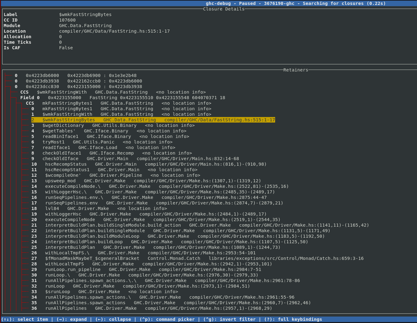
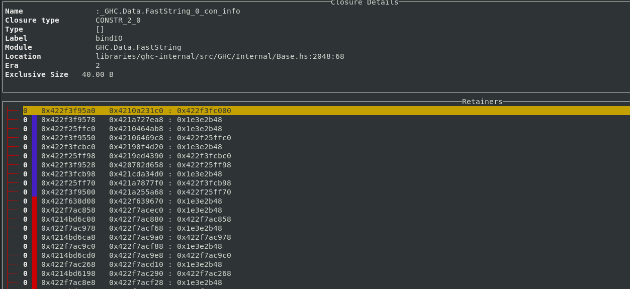
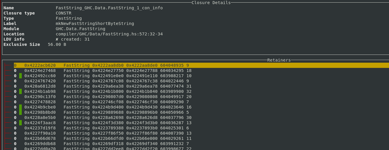
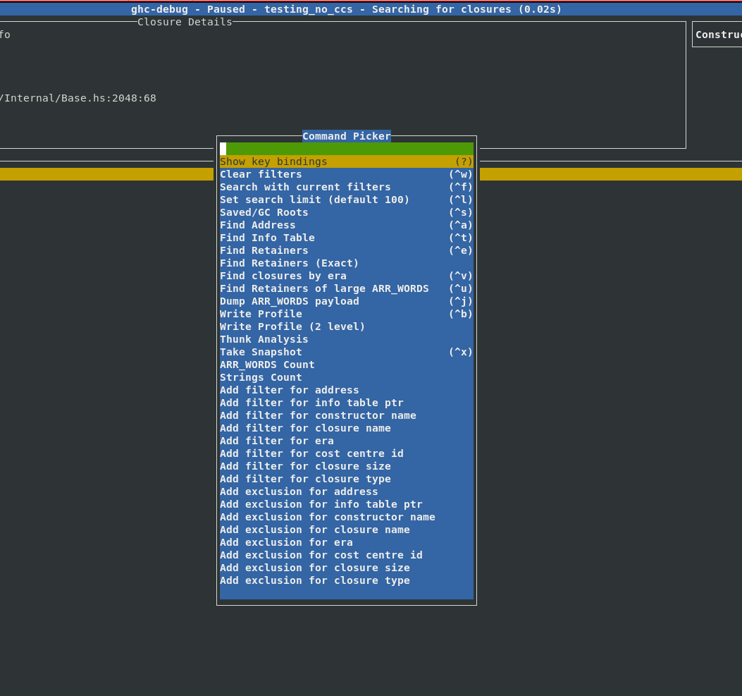
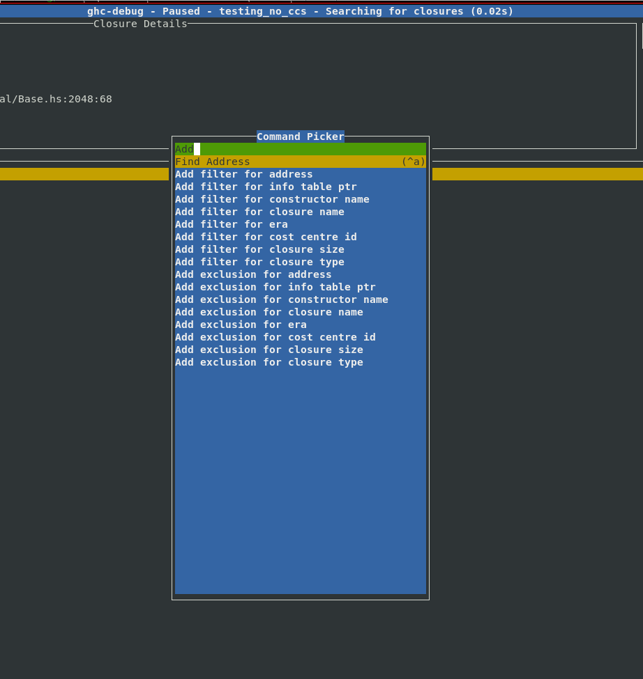
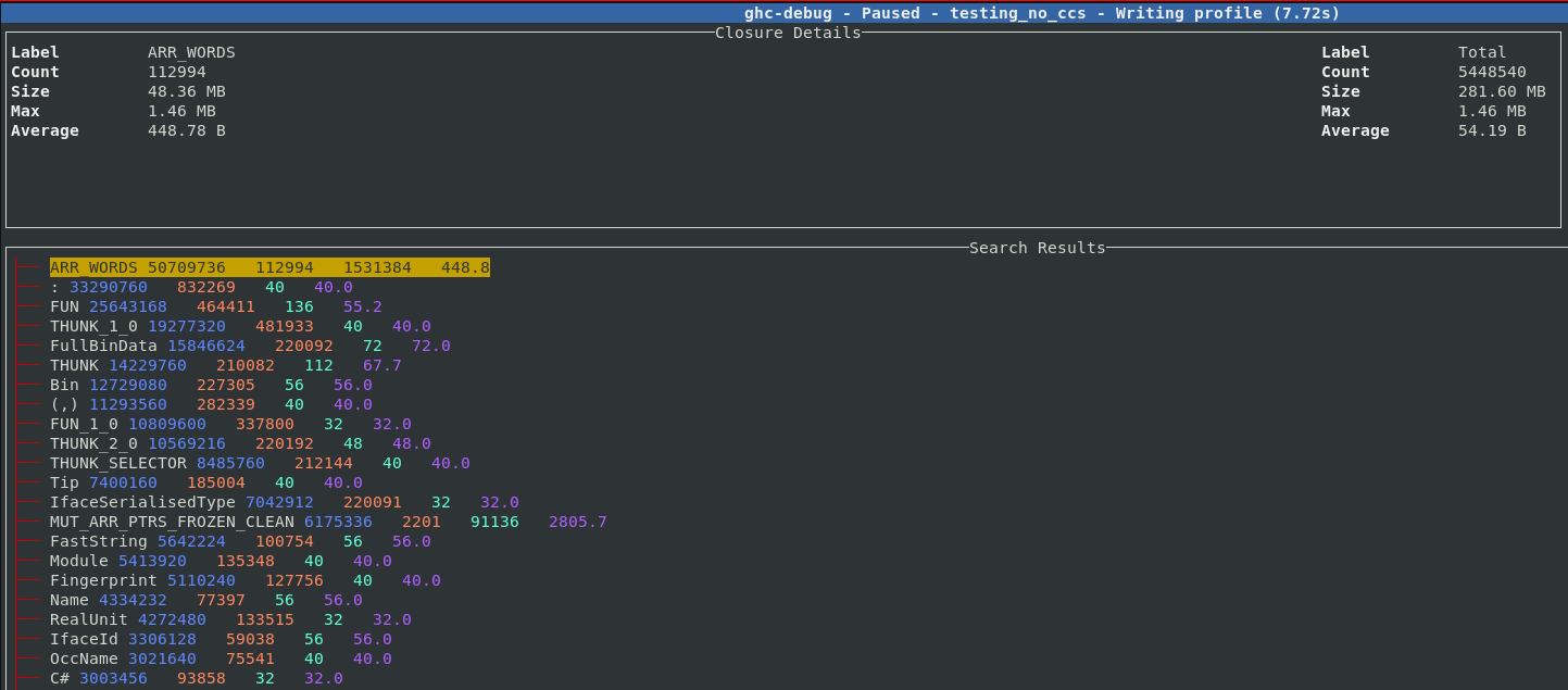
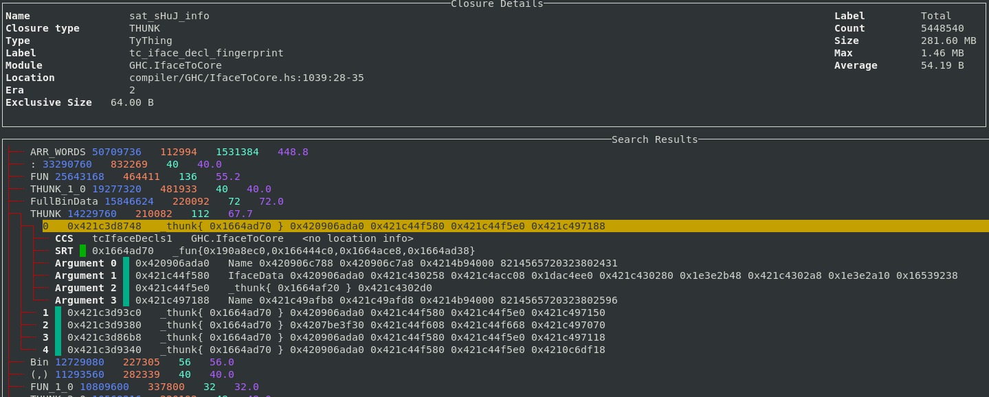
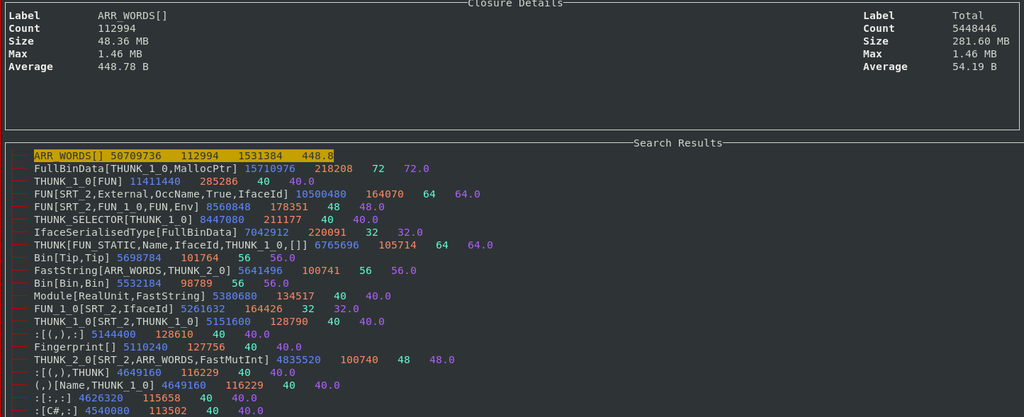
 (a tenth of a full turn). If the shorter edges are of length 1, then the longer edges are of length
  , where
  is the golden ratio.
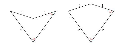
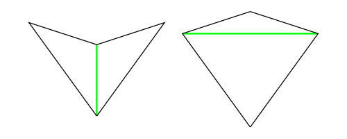
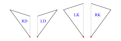
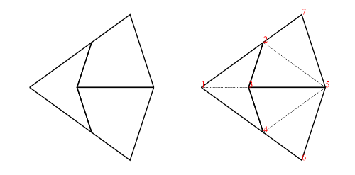
 times the scale of the former, to reflect the change in scale.
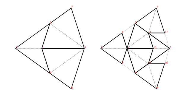
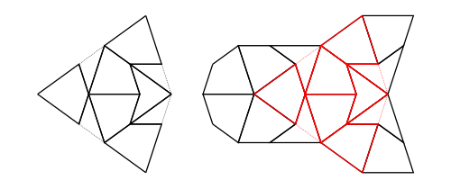
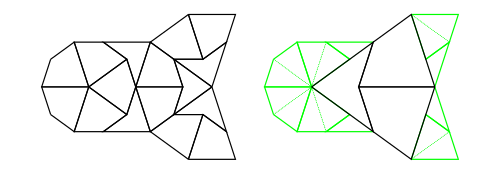
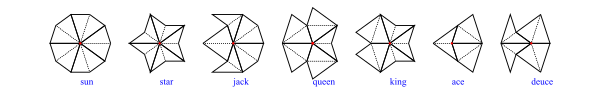
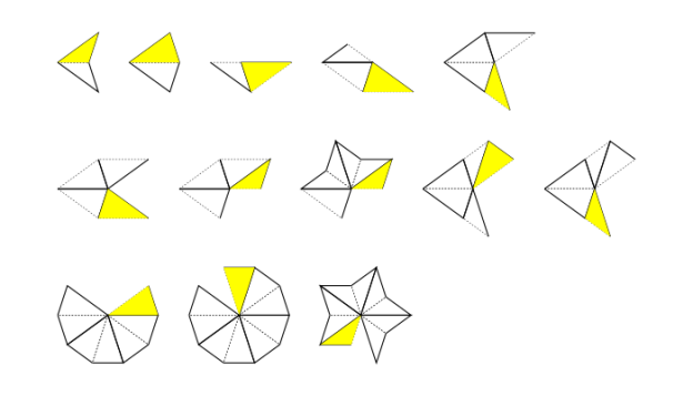
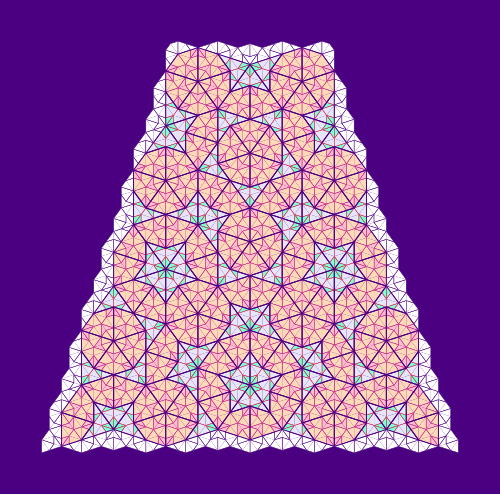


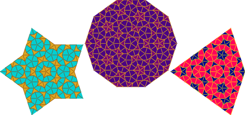
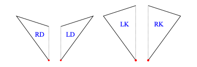
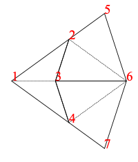
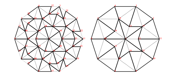
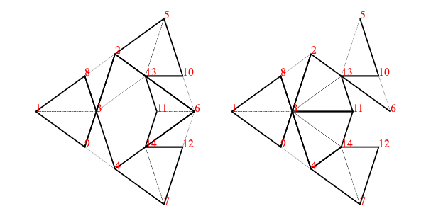
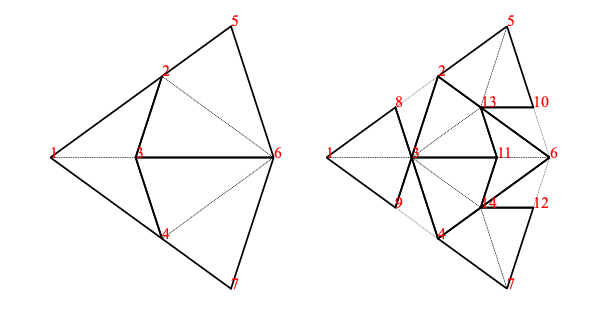
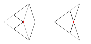
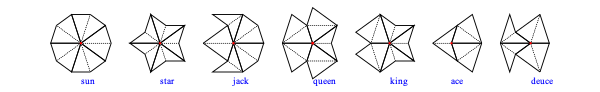
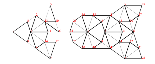
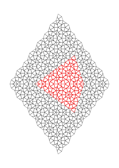
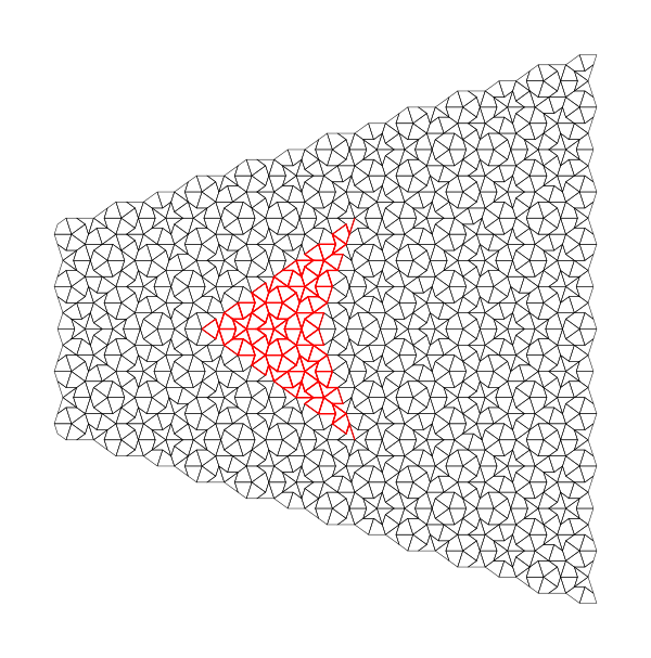
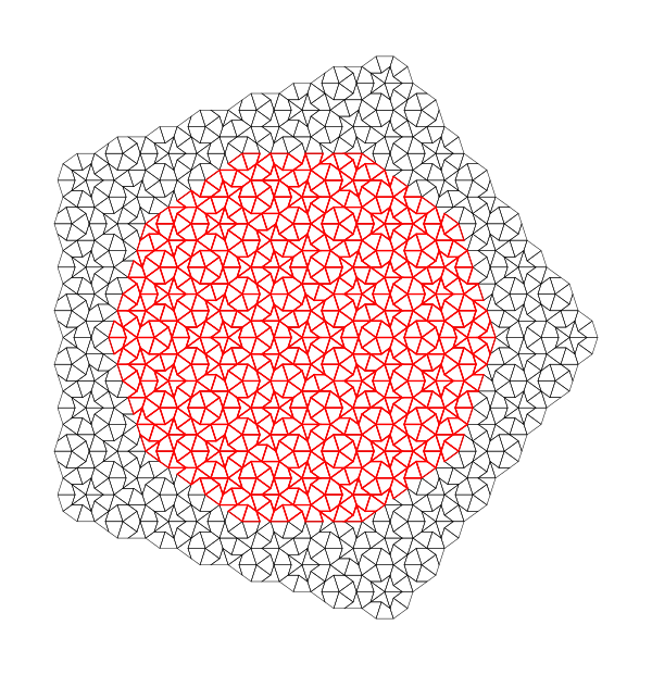
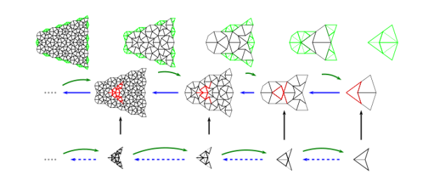
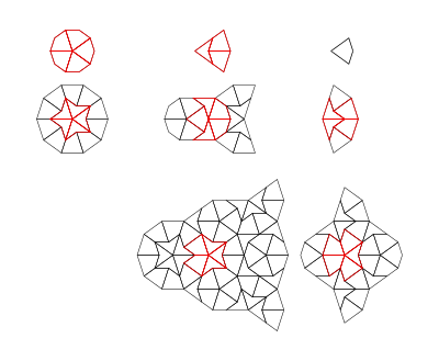
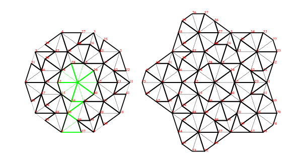


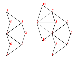
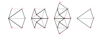
 alternatives for the 2 choices of each of
  unknowns (prior to composing). This uses
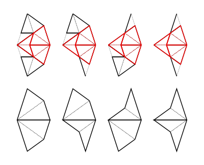
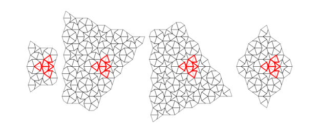


 ,
,  , and
, and  operations along with some proofs.
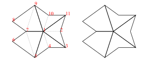

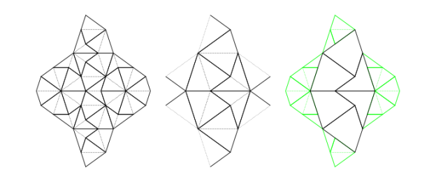
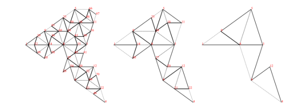
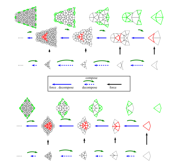
 in these cases. Forcing the decomposition also results in an empty composition. Clearly there is something special about the depicted cases and it is not merely that they are wholetile complete because the decompositions are not wholetile complete. [Wholetile complete means there are no join edges on the boundary, so every half-tile has its other half.]
 and
and  are both valid


 meaning:


 composes perfectly if all faces of

 is a perfect composition if
  composes perfectly.


 is a forced, correct
 using figure 11 (plus an extra case for the forced star). For boundary vertices we check local contexts similar to those depicted in figure 10 (but including empty composition cases). This reveals there is no local change of the boundary at any boundary vertex, and since this is true for all boundary vertices, there can be no global change. (We omit the full details).


 for
for 
 , we have

 for which the composition is defined we have
  so we get
 to get


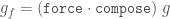 , the right hand side is equivalent to

 (so
(so  ) in the theorem.
  .]
.]


 and so
 and
and  .
. which has lost the leftmost dart of the
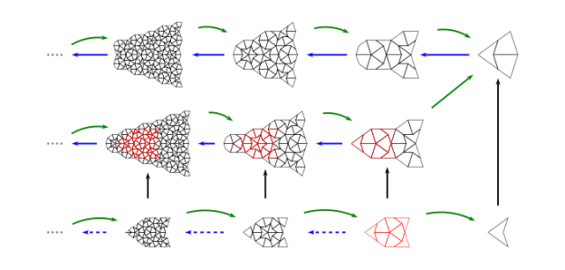
 where
where  , so
, so  ). By the perfect composition theorem we have


 so we have


 is wholetile complete and hence a perfect composition. This means that
  composes perfectly and it is also a generator for
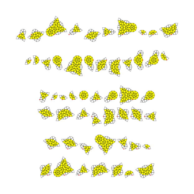
 .
.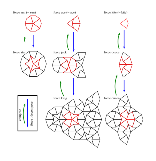
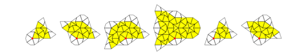
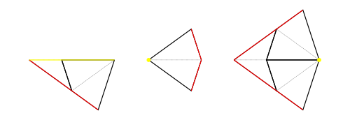
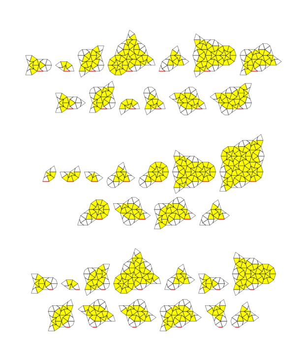


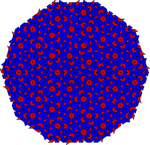
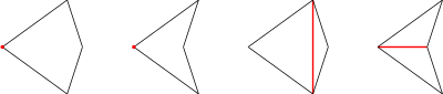
 and so
  ,
,  and
and  .
.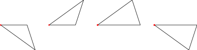

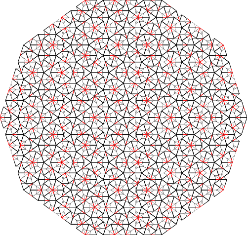
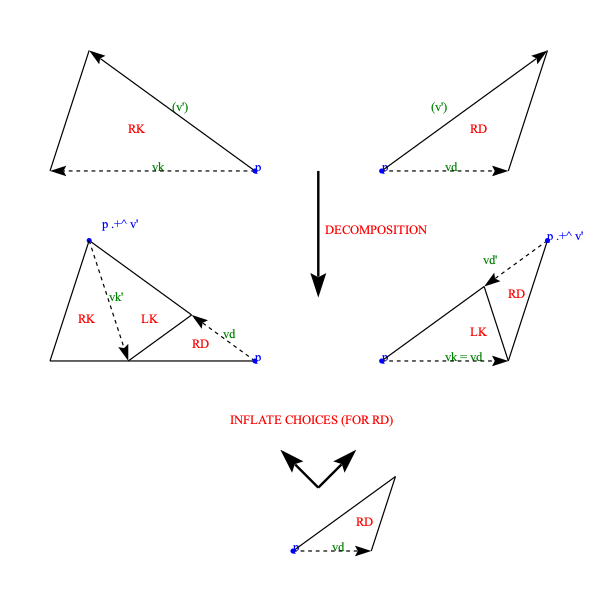
 but we can rescale at any time.)
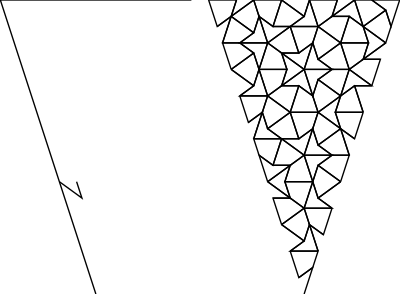
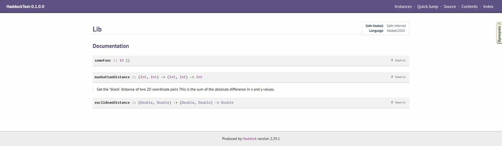
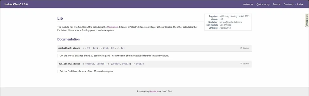


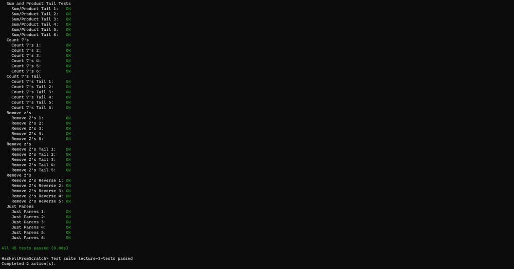

_at_Sassari_station,_Sardinia,_1996.jpg)