Choosing a Computer Language for a Project

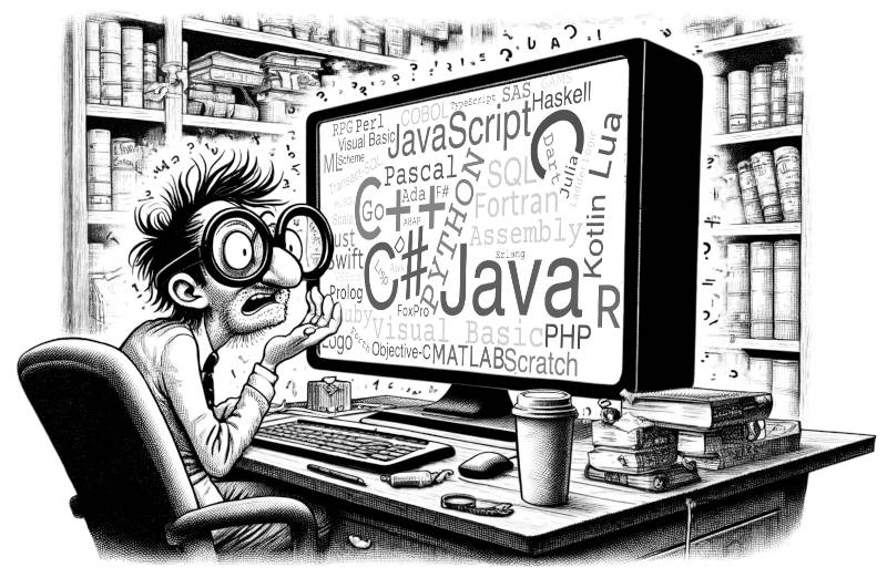
Julia. Scala. Lua. TypeScript. Haskell. Go. Dart. Various computer languages new and old are sometimes proposed as better alternatives to mainstream languages. But compared to mainstream choices like Python, C, C++ and Java (cf. Tiobe Index)—are they worth using?

Certainly it depends a lot on the planned use: is it a one-off small project, or a large industrial-scale software application?

Yet even a one-off project can quickly grow to production-scale, with accompanying growing pains. Startups sometimes face a growth crisis when the nascent code base becomes unwieldy and must be refactored or fully rewritten (or you could do what Facebook/Meta did and just write a new compiler to make your existing code base run better).

The scope of different types of software projects and their requirements is so incredibly diverse that any single viewpoint from experience runs a risk of being myopic and thus inaccurate for other kinds of projects. With this caveat, I’ll share some of my own experience from observing projects for many dozens of production-scale software applications written for leadership-scale high performance computing systems. These are generally on a scale of 20,000 to 500,000 lines of code and often require support of mathematical and scientific libraries and middleware for build support, parallelism, visualization, I/O, data management and machine learning.

Here are some of the main issues regarding choice of programming languages and compilers for these codes:

1. Language and compiler sustainability. While the lifetime of computing systems is measured in years, the lifetime of an application code base can sometimes be measured in decades. Is the language it is written in likely to survive and be well-supported long into the future? For example, Fortran, though still used and frequently supported, is is a less common language thus requiring special effort from vendors, with fewer developer resources than more popular languages. Is there a diversity of multiple compilers from different providers to mitigate risk? A single provider means a single point of failure, a high risk; what happens if the supplier loses funding? Are the language and compilers likely to be adaptable for future computer hardware trends (though sometimes this is hard to predict)? Is there a large customer base to help ensure future support? Similarly, is there an adequate pool of available programmers deeply skilled in the language? Does the language have a well-featured standard library ecosystem and good support for third-party libraries and frameworks? Is there good tool support (debuggers, profilers, build tools)?

2. Related to this is the question of language governance. How are decisions about future updates to the language made? Is there broad participation from the user community and responsiveness to their needs? I’ve known members of the C++ language committee; from my limited experience they seem very reasonable and thoughtful about future directions of the language. On the other hand, some standards have introduced features that scarcely anyone ever uses—a waste of time and more clutter for the standard.

3. Productivity. It is said that programmer productivity is limited by the ability of a few lines of code to express high level abstractions that can do a lot with minimal syntax. Does the language permit this? Does the language standard make sense (coherent, cohesive) and follow the principle of least surprise? At the same time, the language should not engulf what might better be handled modularly by a library. For example, a matrix-matrix product that is bound up with the language might be highly productive for simple cases but have difficulty supporting the many variants of matrix-matrix product provided for example by the NVIDIA CUTLASS library. Also, in-language support for CUDA GPU operations, for example, would make it hard for the language not to lag behind in support of the frequent new releases of CUDA.

4. Strategic advantage. The 10X improvement rule states that an innovation is only worth adopting if it offers 10X improvement compared to existing practice according to some metric . If switching to a given new language doesn’t bring significant improvement, it may not be worth doing. This is particularly true if there is an existing code base of some size. A related question is whether the new language offers an incremental transition path for an existing code to the new language (in many cases this is difficult or impossible).

5. Performance (execution speed). Does the language allow one to get down to bare-metal performance rather than going through costly abstractions or an interpreter layer? Are the features of the underlying hardware exposed for the user to access? Is performance predictable? Can one get a sense of the performance of each line of code just by inspection, or is this occluded by abstractions or a complex compilation process? Is the use of just-in-time compilation or garbage collection unpredictable, which could be a problem for parallel computing wherein unexpected “hangs” can be caused by one process unexpectedly performing one of these operations? Do the compiler developers provide good support for effective and accurate code optimization options?

Early adopters provide a vibrant “early alert” system for new language and tool developments that are useful for small projects and may be broadly impactful. Python was recognized early in the scientific computing community for its potential complementary use with standard languages for large scientific computations. When it comes to planning large-scale software projects, however, a range of factors based on project requirements must be considered to ensure highest likelihood of success.


On greedy algorithms and rodeo clowns

Rodeo clown

This weekend I ran across a blog post The Rodeo Clown Theory of Personal Development. The title comes from a hypothetical example of a goal you don’t know how to achieve: becoming a rodeo clown.

Let’s say you decide you want to be a rodeo clown. And let’s say you’re me and you have no idea how to be a rodeo clown. … Can you look at the possibilities currently available to you and imagine which of them might lead to an overall increase of rodeo clowndom in your life, even infinitesimally?

Each day you ask yourself what you can do that might lead you closer to your goal. This is a greedy algorithm: at each step you make as much progress toward your goal as you can. Greedy algorithms are not always optimal, but the premise above is that you have no idea what to do. In that case, doing whatever you can imagine that might might bring you a little closer to your goal is a smart thing to do.

Crossing the continent

If you’re in Los Angeles and your goal is to get to New York, you could start by walking east. You might run into a brick wall and decide that you should not take your approach too literally. Maybe you decide to buy a ticket for a bus that’s traveling east, even if you have to walk west to the bus station. Maybe the bus takes you to Houston. This isn’t the most direct route, but it’s progress.

When you don’t know what else to do, a greedy approach, especially one tempered with common sense, could be a very sensible way to start. Maybe it’ll put you in a position to learn of a more efficient approach. In the scenario above, maybe some stranger sees you walk into a wall, asks you what you’re trying to do, and tells you where the bus station is.

Sorting algorithms

The way most people sort a hand of playing cards is a sort of greedy algorithm. They scan for the highest card and put it first. Then they scan the remainder of the hand for the next highest card and so on. This algorithm is known as insertion sort. It’s not the most efficient algorithm, but it may be the most natural, and it works. And for a hand of five cards it’s about as good as any.

Anyone who has taken an algorithms class will know you can beat insertion sort with a more sophisticated algorithm such as heap sort. But sorting is a well-understood, one-dimensional problem. That’s why people long ago came up with solutions that are better than a greedy approach. But when a problem is not well understood and is high-dimensional, greedy algorithms are more likely to succeed, even if they’re not optimal.

Training neural nets

Training a neural network is a very high dimensional optimization problem, maybe on the order of a billion dimensions. And yet it is solved using stochastic gradient descent, which is essentially a greedy algorithm. At each iteration, you move in the direction that gives you the most improvement toward your goal. There’s a little more nuance to it than that, but that’s the basic idea.

How can gradient descent work so well in practice when in theory it could get stuck in a local minimum? John Carmack posted a heuristic explanation on Twitter a few weeks ago. A local minimum requires the “cooperation” of every variable in the function you’re optimizing. The more variables, the less likely this is to happen.

Carmack didn’t give a full explanation—he posted a tweet, not a journal article—but he does give an intuitive idea of what’s going on. At the global minimum, the variables cooperate for a good reason. He assumes the variables are unlikely to cooperate anywhere else, which is apparently often true when training neural nets.

Usually things get harder in higher dimensions, hence the “curse of dimensionality.” But there’s a sort of blessing of dimensionality here: you’re less likely to get stuck in a local minimum in higher dimensions.

Back to the rodeo

Training a neural network can be a huge undertaking, using millions of dollars worth of electricity, but it’s a mathematically defined problem. Life goals such as becoming a rodeo clown are not cleanly quantified problems. They are very high dimensional in the sense that there are a vast number of things you could do at any given time. You might argue by analogy with neural nets that the fact that there are so many dimensions means that you’re unlikely to get stuck in a local minimum. This is a loose analogy, one that easily breaks down, but still one worth thinking about.

Seth Godin once said “Remarkable work often comes from making choices when everyone else feels as though there is no choice.” What looks like a local minimum may be revealed to not be once you consider more options.


Image by Clarence Alford from Pixabay

Finding strings in binary files

There’s a little program called strings that searches for what appear to be strings inside binary file. I’ll refer to it as strings(1) to distinguish the program name from the common English word strings. [1]

What does strings(1) consider to be a string? By default it is a sequence of four or more bytes that correspond to printable ASCII strings. There are command options to change the sequence length and the character encoding.

There are 98 printable ASCII characters [2] and 256 possible values for an 8-bit byte, so the probability of a byte being a printable character is

p = 98/256 = 0.3828125.

This implies that the probability of strings(1) flagging a sequence of four random bytes as a string is p4 or about 2%.

How long a string might you find inside a binary file?

I ran strings(1) on a photograph and found a 46-character string:

   .IEC 61966-2.1 Default RGB colour space - sRGB

Of course this isn’t random. This string is part of the metadata stored inside JPEG images.

Next I encrypted the file so that no strings would be metadata and all strings would be false positives. The longest line was 12 characters:

    Z<Bq{7fH}~G9

How does this compare to what we might expect from a random file? I wrote about the probability of long runs a dozen years ago. In a file of n bytes, the expected length of the longest run of printable characters is approximately

-frac{log n(1-p)}{log p}

In my case, the file had n = 203,308 bytes. The expected length of the longest run of printable characters would then be 12.2 characters, and so the actual length of the longest run is in line with what theory would have predicted.


[1] Unix documentation is separated into sections, and parentheses after a name specify the documentation section. Section 1 is for programs, Section 2 is for system calls, etc. So, for example, chmod(1) is the command line utility named chmod, and chmod(2) is the system call by the same name. Since command line utilities often have names that are common words, tacking (1) on the end helps distinguish program names from English words.

[2] p could be a little larger if you consider some of the control characters to be printable.

Extract text from a PDF

Arshad Khan left a comment on my post on the less and more utilities saying “on ubuntu if I do less on a pdf file, it shows me the text contents of the pdf.”

Apparently this is an undocumented feature of GNU less. It works, but I don’t see anything about it in the man page documentation [1].

Not all versions of less do this. On my Mac, less applied to a PDF gives a warning saying “… may be a binary file. See it anyway?” If you insist, it will dump gibberish to the command line.

A more portable way to extract text from a PDF would be to use something like the pypdf Python module:

    from pypdf import PdfReader

    reader = PdfReader("myfile.pdf")
    for page in reader.pages:
        print(page.extract_text()) 

The pypdf documentation gives several options for how to extract text. The documentation also gives a helpful discussion of why it’s not always clear what extracting text from a PDF should mean. Should captions and page numbers be extracted? What about tables? In what order should text elements be extracted?

PDF files are notoriously bad as a data exchange format. When you extract text from a PDF, you’re likely not using the file in a way its author intended, maybe even in a way the author tried to discourage.

Related post: Your PDF may reveal more than you intend

[1] Update: Several people have responded saying that that less isn’t extracting the text from a PDF, but lesspipe is. That would explain why it’s not a documented feature of less. But it’s not clear how lesspipe is implicitly inserting itself.

Further update: Thanks to Konrad Hinsen for pointing me to this explanation. less reads an environment variable LESSOPEN for a preprocessor to run on its arguments, and that variable is, on some systems, set to lesspipe.

Length of a general Archimedean spiral

This post ties together the previous three posts.

In this post, I said that an Archimedean spiral has the polar equation

r = b θ1/n

and applied this here to rolls of carpet.

When n = 1, the length of the spiral for θ running from 0 to T is approximately

½ bT²

with the approximation becoming more accurate [1] as T increases.

In this post we want to look at the general case where n might not be 1. In that case the arc length is given by a hypergeometric function, and finding the asymptotic behavior for large T requires evaluating a hypergeometric function at a large argument.

Here’s an example with n = 3.

Now the arms are not equally spaced but instead grow closer together.

Arc length

According to MathWorld, the length of the spiral with n > 1 and θ running from 0 to T is given by

L = b T^{1/n} \,_2F_1\left(-\frac{1}{2}, \frac{1}{2n}; 1 + \frac{1}{2n}; -n^2 T^2 \right)

As I discussed here, the power series defining a hypergeometric function 2F1 diverges for arguments outside the unit disk, but the function can be extended by analytic continuation using the identity

\begin{align*} F(a, b; c; z) &= \frac{\Gamma(c) \Gamma(b-a)}{\Gamma(b) \Gamma(c-a)} \,(-z)^{-a\phantom{b}} F\left(a, 1-c+a; 1-b+a; \frac{1}{z}\right) \\ &+ \frac{\Gamma(c) \Gamma(a-b)}{\Gamma(a) \Gamma(c-b)} \,(-z)^{-b\phantom{a}} F\left(\,b, 1-c+b; 1-a+b; \,\frac{1}{z}\right) \\ \end{align*}

Asymptotics

Most of the terms above will drop out in the limit as z = −n²T² gets large. The 1/z terms go to zero, and hypergeometric functions equal 1 when z = 0, and so the F terms on the right hand side above go to 1 as T increases.

In our application the hypergeometric parameters are a = −1/2, b = 1/2n, and c = 1 + 1/2n. The term

(−z)a  = (−z)1/2

matters, but the term

(−z)b  = (−z)−1/2n

goes to zero and can be ignored.

We find that

Lk T1 + 1/n

where the constant k is given by

k = bn Γ(1 + 1/2n) Γ(1/2 + 1/2n) / Γ(1/2n) Γ(3/2 + 1/2n)

When n = 1, this reduces to L ≈ ½ bT² as before.


[1] The relative approximation error decreases approximately quadratically in T. But the absolute error grows algorithmically.

How big will a carpet be when you roll or unroll it?

If you know the dimensions of a carpet, what will the dimensions be when you roll it up into a cylinder?

If you know the dimensions of a rolled-up carpet, what will the dimensions be when you unroll it?

This post answers both questions.

Flexible carpet: solid cylinder

The edge of a rolled-up carpet can be described as an Archimedian spiral. In polar coordinates, this spiral has the equation

r = hθ / 2π

where h is the thickness of the carpet. The previous post gave an exact formula for the length L of the spiral, given the maximum value of θ which we denoted T. It also gave a simple approximation that is quite accurate when T is large, namely

L = hT² / 4π

If r1 is the radius of the carpet as a rolled up cylinder, r1 = hT / 2π and so T = 2π r1 / h. So when we unroll the carpet

L = hT² / 4π = πr1² / h.

Now suppose we know the length L and want to find the radius r when we roll up the carpet.

T = √(hL/π).

Stiff carpet: hollow cylinder

The discussion so far has assumed that the spiral starts from the origin, i.e. the carpet is rolled up so tightly that there’s no hole in the middle. This may be a reasonable assumption for a very flexible carpet. But if the carpet is stiff, the rolled up carpet will not be a solid cylinder but a cylinder with a cylindrical hole in the middle.

In the case of a hollow cylinder, there is an inner radius r0 and an outer radius r1. This means θ runs from T0 = 2π r0/h to T1 = 2πr1/h.

To find the length of the spiral running from T to T1 we find the length of a spiral that runs from 0 to T1 and subtract the length of a spiral from 0 to T0

L = πr1² / h − πr0² / h = π(r1² − r0²)/h.

This approximation is even better because the approximation is least accurate for small T, and we’ve subtracted off that part.

Now let’s go the other way around and find the outer radius r1 when we know the length L. We also need to know the inner radius r0. So suppose we are wrapping the carpet around a cardboard tube of radius r0. Then

r1 = √(r0² + hL/π).

Approximating a spiral by rings

An Archimedean spiral has the polar equation

r = b θ1/n

This post will look at the case n = 1. I may look at more general values of n in a future post. (Update: See here.) The case n = 1 is the simplest case, and it’s the case I needed for the client project that motivated this post.

In this case the spacing between points where the spiral crosses an axis is constant. Call this constant h. Then

h = 2πb.

For example, when rolling up a carpet, h corresponds to the thickness of the carpet.

Suppose θ runs from 0 to 2πm, wrapping around the origin m times. We could approximate the spiral by m concentric circles of radius h, 2h, 3h, …, mh. To visualize this, we’re approximating the length of the red spiral on the left with that of the blue circles on the right.

Comparing Archimedes spiral and concentric circles

We could approximate this further by saying we have m/2 circles whose average radius is πmb. This suggests the length of the spiral should be approximately

2π²m²b

How good is this approximation? What happens to the relative error as θ increases? Intuitively, each wrap around the origin is more like a circle as θ increases, so we’d expect the approximation to improve for large θ.

According to Mathworld, the exact length of the spiral is

πbm √(1 + (2πm)²) + b arcsinh(2πm) /2

When m is so large that we can ignore the 1 in √(1 + (2πm)²) then the first term is the same as the circle approximation, and all that’s left is the arcsinh term, which is on the order of log m because

arcsinh(x) = log(x + (1 + x²)1/2).

So for large m, the arc length is on the order of m² while the error is on the order of log m. This means the relative error is O( log(m) / m² ). [1]

We’ve assumed m was an integer because that makes it easier to visual approximating the spiral by circles, but that assumption is not necessary. We could restate the problem in terms of the final value of θ. Say θ runs from 0 to T. Then we could solve

T = 2πm

for m and say that the approximate arc length is

½ bT²

and the exact length is

½ bT(1 + T²)1/2 + ½ b arcsinh(T).

The relative approximation error is O( log(T) / T² ).

Here’s a plot of the error as a function of T assuming b = 1.

Related posts

[1] The error in approximating √(1 + (2πm)²) with 2πm is on the order of 1/(4πm) and so is smaller than the logarithmic term.

Hypergeometric function of a large negative argument

It’s occasionally necessary to evaluate a hypergeometric function at a large negative argument. I was working on a project today that involved evaluating F(a, b; c; z) where z is a large negative number.

The hypergeometric function F(a, b; c; z) is defined by a power series in z whose coefficients are functions of a, b, and c. However, this power series has radius of convergence 1. This means you can’t use the series to evaluate F(a, b; c; z) for z < −1.

It’s important to keep in mind the difference between a function and its power series representation. The former may exist where the latter does not. A simple example is the function f(z) = 1/(1 − z). The power series for this function has radius 1, but the function is defined everywhere except at z = 1.

Although the series defining F(a, b; c; z) is confined to the unit disk, the function itself is not. It can be extended analytically beyond the unit disk, usually with a branch cut along the real axis for z ≥ 1.

It’s good to know that our function can be evaluated for large negative x, but how do we evaluate it?

Linear transformation formulas

Hypergeometric functions satisfy a huge number of identities, the simplest of which are known as the linear transformation formulas even though they are not linear transformations of z. They involve bilinear transformations z, a.k.a. fractional linear transformations, a.k.a. Möbius transformations. [1]

One such transformation is the following, found in A&S 15.3.4 [2].

F(a, b; c; z) = (1-z)^{-a} F\left(a, c-b; c; \frac{z}{z-1} \right)

If z < 1, then 0 < z/(z − 1) < 1, which is inside the radius of convergence. However, as z goes off to −∞, z/(z − 1) approaches 1, and the convergence of the power series will be slow.

A more complicated, but more efficient, formula is A&S 15.3.7, a linear transformation formula relates F at z to two other hypergeometric functions evaluated at 1/z. Now when z is large, 1/z is small, and these series will converge quickly.

\begin{align*} F(a, b; c; z) &= \frac{\Gamma(c) \Gamma(b-a)}{\Gamma(b) \Gamma(c-a)} \,(-z)^{-a\phantom{b}} F\left(a, 1-c+a; 1-b+a; \frac{1}{z}\right) \\ &+ \frac{\Gamma(c) \Gamma(a-b)}{\Gamma(a) \Gamma(c-b)} \,(-z)^{-b\phantom{a}} F\left(\,b, 1-c+b; 1-a+b; \,\frac{1}{z}\right) \\ \end{align*}

Related posts

[1] It turns out these transformations are linear, but not as functions of a complex argument. They’re linear as transformations on a projective space. More on that here.

[2] A&S refers to the venerable Handbook of Mathematical Functions by Abramowitz and Stegun.

More is less

When I first started using Unix, I used a program called “more” to read files. The name makes sense because each time you press the space bar, more will show you more of your file, one screen at a time.

Now everyone uses less, and more is all but forgotten.

Daniel Halbert wrote more in 1978. Mark Nudelman a similar program with more functionality in 1984 which he named less. The name was a pun on the aphorism “less is more” [1]. Soon less completely replaced more.

I’m curious why I ever used more, since less had taken over before I touched Unix. One possibility is that someone who was accustomed to more showed me that command. Another possibility is that I learned it from reading The Unix Programming Environment which came out in November 1983. It includes more but not less.

My laptop contains executables for more and less in /usr/bin. The command

    diff less more

returns nothing, indicating that the binaries are identical: less literally is more.

My desktop has distinct binaries for less and more. The more binary is much smaller, and so I assume it is limited to the original functionality of more, more or less.

Related posts

[1] I don’t know who coined the phrase “less is more,” but it is associated with architect Ludwig Mies van der Rohe (1886–1969) who often quoted it. He did not apply the principle to is own name, however. He was born Ludwig Mies and later appended van der Rohe.

Precise answers to useless questions

I recently ran across a tweet from Allen Downey saying

So much of 20th century statistics was just a waste of time, computing precise answers to useless questions.

He’s right. I taught mathematical statistics at GSBS [1, 2] several times, and each time I taught it I became more aware of how pointless some of the material was.

I do believe mathematical statistics is useful, even some parts whose usefulness isn’t immediately obvious, but there were other parts of the curriculum I couldn’t justify spending time on [3].

Fun and profit

I’ll say this in partial defense of computing precise answers to useless questions: it can be fun and good for your career.

Mathematics problems coming out of statistics can be more interesting, and even more useful, than the statistical applications that motivate them. Several times in my former career a statistical problem of dubious utility lead to an interesting mathematical puzzle.

Solving practical research problems in statistics is hard, and can be hard to publish. If research addresses a practical problem that a reviewer isn’t aware of, a journal may reject it. The solution to a problem in mathematical statistics, regardless of its utility, is easier to publish.

Private sector

Outside of academia there is less demand for precise answers to useless questions. A consultant can be sure that a client finds a specific project useful because they’re willing to directly spend money on it. Maybe the client is mistaken, but they’re betting that they’re not.

Academics get grants for various lines of research, but this isn’t the same kind of feedback because the people who approve grants are not spending their own money. Imagine a grant reviewer saying “I think this research is so important, I’m not only going to approve this proposal, I’m going to write the applicant a $5,000 personal check.”

Consulting clients may be giving away someone else’s money too, but they have a closer connection to the source of the funds than a bureaucrat has when dispensing tax money.

Notes

[1] When I taught there, GSBS was The University of Texas Graduate School of Biomedical Sciences. I visited their website this morning, and apparently GSBS is now part of, or at least co-branded with, MD Anderson Cancer Center.

There was a connection between GSBS and MDACC at the time. Some of the GSBS instructors, like myself, were MDACC employees who volunteered to teach a class.

[2] Incidentally, there was a connection between GSBS and Allen Downey: one of my students was his former student, and he told me what a good teacher Allen was.

[3] I talk about utility a lot in this post, but I’m not a utilitarian. There are good reasons to learn things that are not obviously useful. But the appeal of statistics is precisely its utility, and so statistics that isn’t useful is particularly distasteful.

Pure math is beautiful (and occasionally useful) and applied math is useful (and occasionally beautiful). But there’s no reason to study fake applied math that is neither beautiful or useful.